O(3), Spherical Harmonics, and Cartesian Tensors
Please Log In for full access to the web site.
Note that this link will take you to an external site (https://shimmer.mit.edu) to authenticate, and then you will be redirected back to this page.
These notes are being transcribed, condensed, and illustrated. They may lag or omit details, please refer to the handwritten notes for the full lecture.
1) Introduction and Roadmap
In the Lie groups notes we studied \mathrm{SO}(2) and \mathrm{SO}(3) — the groups of pure rotations in 2D and 3D. But the full symmetry of many of the point groups we've studied in this course, and of Euclidean space itself, includes more than just rotations (and translations, for the Euclidean group): it also includes reflections and inversions. Adding these parity operations to \mathrm{SO}(n) gives the orthogonal group O(n).
In this note we ask: what happens to our representation theory when we extend from \mathrm{SO}(n) to O(n)? Parity (\mathbb{Z}_2) is the simplest possible group — just two elements — and yet it impacts the irreps of \mathrm{SO}(2) and \mathrm{SO}(3) in interestingly different ways:
- In O(2), the m = 0 irrep of \mathrm{SO}(2) splits into a scalar (+1 for all elements) and a pseudoscalar (-1 for reflections/mirrors). For m \geq 1, the reflection mixes e^{+im\alpha} and e^{-im\alpha}, so they can no longer be separate irreps — instead they combine into 2D real irreps labeled by positive integer m.
- In O(3), inversion commutes with rotations, so the structure is simpler: each \mathrm{SO}(3) irrep just gets a parity label (\pm 1), giving pairs like vectors vs. pseudovectors that rotate identically but differ under inversion. The irreps of O(3) are labeled by angular momentum l and parity p.
What does understanding O(3) tell us about the point groups we've been studying? Every 3D point group is a subgroup of O(3), so we can ask how O(3) irreps branch (decompose) under point groups — this is pure representation theory, requiring only QS = RQ.
Similarly, we can construct basis functions for the irreps of O(2) and O(3) — circular harmonics (\cos(m\theta), \sin(m\theta)) for O(2), and spherical harmonics (Y_l^m(x,y,z)) for O(3) — and then ask how these functions branch under point groups. Combining branching with these polynomial basis functions finally explains the "linear functions," "quadratic functions," and "rotation" columns of character tables.
We then extend this analysis to Cartesian tensors — physical quantities whose index symmetries further constrain which irreps appear — and show how decomposing into O(3) irreps combined with branching determines the independent components of physical tensors like the elasticity tensor. Finally, we connect to power spectra and bispectra of spherical signals, and show how group symmetry predicts which spectral components vanish.
2) From \mathrm{SO}(n) to O(n): Adding Parity
2.1) O(2): A Semi-Direct Product
The group O(2) is the full symmetry group of 2D Euclidean space (modulo translations). It includes both rotations and reflections:
where \mathbb{Z}_2 = \{I, M_x\} consists of the identity and a mirror reflection. In the \{x, y\} basis, M_x = \begin{pmatrix} 1 & 0 \\ 0 & -1 \end{pmatrix} (reflects across the x-axis). This is not the only choice of mirror — any U M_x U^{-1} (a reflection across a different axis) would work equally well. This is a semi-direct product (\rtimes) because rotations and mirrors do not commute. For example, with R(90°) = \begin{pmatrix} 0 & -1 \\ 1 & 0 \end{pmatrix}:
Both are reflections, but across different axes — the order matters.
Recall from the Lie groups notes that the irreps of \mathrm{SO}(2) are the complex 1D representations e^{im\alpha} for integer m. A mirror sends a rotation by \alpha to a rotation by -\alpha, so it maps e^{im\alpha} \mapsto e^{-im\alpha}. This means the mirror swaps the +m and -m irreps. What does this do to the representation theory?
-
m = 0: The trivial representation e^{i \cdot 0 \cdot \alpha} = 1 is unchanged by the mirror — but we can still ask how the mirror itself is represented. This gives two 1D irreps:
- Trivial (
0e): D(g) = 1 for all g \in O(2) - Pseudoscalar (
0o): D(g) = 1 for rotations, D(g) = -1 for reflections
- Trivial (
-
m \geq 1: Since the mirror swaps e^{+im\alpha} and e^{-im\alpha}, neither can be an irrep on its own — the mirror would take you out of the representation. Instead, +m and -m must pair up into a single 2D real irrep. Taking real and imaginary parts of e^{\pm im\alpha} gives the familiar 2 \times 2 rotation matrices:
Key insight for O(2): Adding a mirror to \mathrm{SO}(2) forces the complex conjugate pair e^{\pm im\alpha} to merge into a single real 2D irrep — this is why the "standard" 2D rotation matrices appear. They aren't just a convenient choice of basis; they are the only irreps once reflections are included. The \cos/\sin form emerges from choosing the representation to be real and closed under the mirror.
Selection rule for O(2): the O(2) irreps are labeled by positive integers m = 1, 2, 3, \ldots (plus the two 1D irreps at m = 0). The tensor product selection rule is m_3 = |m_1 \pm m_2| — both + and - are possible, unlike \mathrm{SO}(2) where the old (signed) m only allowed m_3 = m_1 + m_2. The - branch appears because the +m and -m of \mathrm{SO}(2) are now combined into a single irrep, so both sums are accessible within one tensor product.
2.2) O(3): A Direct Product
In 3D, something different happens. The parity operation is inversion \mathcal{I} = -I_3 (flip all three axes), and unlike the 2D mirror, inversion commutes with every rotation: \mathcal{I} R = R \mathcal{I} (because -I commutes with any matrix). This means:
This is a direct product (\times), not a semi-direct product. The consequence for representation theory is much simpler than O(2): since the groups commute, the irreps of the direct product are simply the tensor products of irreps of the individual groups. Each \mathrm{SO}(3) irrep (labeled by l) gets paired with each \mathbb{Z}_2 irrep (p = +1 or p = -1), giving two versions of every angular momentum level.
Irreps of O(3) are labeled by two indices: angular momentum l from \mathrm{SO}(3) and parity p \in \{+1, -1\} from \mathbb{Z}_2. The dimension remains 2l + 1. Under a rotation R \in \mathrm{SO}(3), the irrep acts as D^{(l)}(R). Under inversion, the irrep acts as p \cdot \mathbb{1}_{2l+1}.
Contrast with O(2): In O(2), the mirror mixed different \mathrm{SO}(2) irreps (+m and -m got glued together into 2D real irreps). In O(3), inversion doesn't mix anything — each \mathrm{SO}(3) irrep just acquires a parity label. The resulting pairs (e.g. vectors 1o vs. pseudovectors 1e) rotate identically under \mathrm{SO}(3) but differ in their behavior under inversion. You cannot tell them apart by rotations alone — only inversion (or a reflection, which is inversion composed with a rotation) distinguishes them.
Commonly encountered O(3) irreps (using the e3nn shorthand Lp where e = even parity, o = odd):
| Label | l | p | Dim | Physical example |
|---|---|---|---|---|
0e |
0 | +1 | 1 | scalar (energy, charge) |
0o |
0 | -1 | 1 | pseudoscalar (chirality) |
1o |
1 | -1 | 3 | vector (position, force) |
1e |
1 | +1 | 3 | pseudovector (angular momentum, magnetic field) |
2e |
2 | +1 | 5 | symmetric traceless tensor (quadrupole, strain) |
2o |
2 | -1 | 5 | pseudo-rank-2 tensor |
2.3) Selection Rules for O(3)
The tensor product selection rules for O(3) combine the \mathrm{SO}(3) triangle rule with parity multiplication:
The parity rule follows from \mathbb{Z}_2 multiplication:
| p_1 | p_2 | p_3 |
|---|---|---|
| even | even | even |
| even | odd | odd |
| odd | even | odd |
| odd | odd | even |
For example, 1o \otimes 1o = 0e \oplus 1e \oplus 2e (two odd vectors give even-parity outputs).
2.4) Working with O(3) Computationally
While \mathrm{SO}(3) forms a Lie group (and we work with generators), \mathbb{Z}_2 does not. To decompose representations under O(3), we use representations (not generators) evaluated at random 3D rotoinversions. Why do random samples work? The constraint QS(g) = R(g)Q must hold for all group elements g \in O(3). If we sample g randomly, we are unlikely to accidentally pick only elements that generate a subgroup — with good coverage, the random samples are just as constraining as the full continuous group. In practice, 10–20 random rotoinversions are more than sufficient.
In the SO(3) and O(3) exercise, you will implement a function that constructs O(3) irreps:
o3_irrep = so3.o3_irrep(so3_irreps[L], rot_params, sign_params, parity=p)
This constructs the O(3) irrep with angular momentum L and parity p by exponentiating the \mathrm{SO}(3) generators at sampled rotation parameters, then multiplying by p^{\text{sign}} to incorporate the inversion. Once you have O(3) irreps as explicit matrices (not generators), you can use infer_change_of_basis and rep.tensor_product as usual.
3) Branching Under Point Groups
Every 3D point group (C_{2v}, T_d, O_h, etc.) is a subgroup of O(3). This means every irrep of O(3), when restricted to only the elements of a point group, must decompose into a direct sum of irreps of that point group. This decomposition is called branching (or subduction).
Branching is computed using QS = RQ: set S to be the O(3) irrep restricted to the subgroup elements, and R to each point group irrep in turn. The dimension of the solution space gives the multiplicity. This is the same change-of-basis computation we've used throughout the course — no new machinery is needed.
In code, this is exactly what vib_modes.branching_change_of_basis does:
# Here o3_irreps have been evaluated at all |G| subgroup elements,
# so the subgroup element indices are simply np.arange(len(sub)).
branch = vib_modes.branching_change_of_basis(o3_irreps, sub_irreps, np.arange(len(sub)))
# branch[i][j] is the change-of-basis matrix from O(3) irrep i to point group irrep j
# branch[i][j].shape[0] gives the multiplicity
Note that branching is purely about representations — we don't need basis functions (spherical harmonics) to compute it. We just need the irrep matrices of O(3) and of the point group.
3.1) Example: Branching Under T_d
The tetrahedral group T_d has irreps A_1, A_2, E, T_1, T_2 (dimensions 1, 1, 2, 3, 3). Using the o3_branch helper function:
| O(3) irrep | A_1 | A_2 | E | T_1 | T_2 |
|---|---|---|---|---|---|
0e |
1 | ||||
0o |
1 | ||||
1e |
1 | ||||
1o |
1 | ||||
2e |
1 | 1 | |||
2o |
1 | 1 | |||
3e |
1 | 1 | 1 | ||
3o |
1 | 1 | 1 |
This table tells us, for example, that the l = 2 (even parity) representation of O(3) splits into the E (2D) and T_2 (3D) irreps of T_d: 2e \to E \oplus T_2.
4) Basis Functions: Circular and Spherical Harmonics
4.1) Circular Harmonics: Basis Functions for O(2)
Before constructing spherical harmonics for O(3), notice that we've already seen their 2D analog: the \cos(m\theta) and \sin(m\theta) functions that appear in the O(2) irreps (§2.1) are circular harmonics — polynomial basis functions on the unit circle.
For each m \geq 1, the pair \{\cos(m\theta), \sin(m\theta)\} forms a basis for the 2D irrep of O(2) with "angular frequency" m. These are the lowest-order trigonometric polynomials that transform as that irrep. Equivalently, in Cartesian coordinates on the unit circle (x = \cos\theta, y = \sin\theta), circular harmonics are homogeneous polynomials of degree m in (x, y) restricted to x^2 + y^2 = 1:
- m = 1: \{x, y\} (the coordinates themselves — the vector representation)
- m = 2: \{x^2 - y^2, 2xy\} (the "quadrupole" patterns)
- m = 3: \{x^3 - 3xy^2, 3x^2y - y^3\}
The parallel to O(3) is exact: circular harmonics are to O(2) what spherical harmonics are to O(3) — both are the lowest-order polynomial basis functions for each irrep of the rotation group, restricted to the unit sphere (circle in 2D, sphere in 3D).
Note that the m = 0 scalar (trivial irrep) has the constant basis function 1, but the m = 0 pseudoscalar has no polynomial basis function in \{x, y\} — it is a representation that assigns +1 to rotations and -1 to reflections, with no angular dependence to visualize. (This is analogous to how pseudovectors in O(3) have no polynomial basis in a single coordinate.)
The interactive graphic below shows the circular harmonics for m = 1 through m = 4, visualized as polar plots where the radius indicates the magnitude and the color indicates the sign (purple for positive, yellow for negative):
4.2) Spherical Harmonics as Basis Functions
Spherical harmonics Y_l^m(\hat{\mathbf{r}}) are the lowest order polynomials of a 3D point \{x, y, z\} that transform as irreps of \mathrm{SO}(3) (or O(3)), restricted to the unit sphere r = 1. They can be constructed using Clebsch-Gordan coefficients from tensor products.
Why restrict to the sphere? A polynomial like x^2 - y^2 is a function of all three coordinates, but its transformation under rotation depends only on the angular part — not on r = \sqrt{x^2 + y^2 + z^2}. Since rotation preserves r (it's invariant), we can factor any homogeneous polynomial into a radial part r^l times an angular part that lives on the unit sphere: p(x,y,z) = r^l \, Y_l^m(\hat{\mathbf{r}}). The radial part carries no representation information, so we can set r = 1 (or equivalently, normalize by dividing by r^l) without losing any information about how the function transforms. This is why spherical harmonics are defined on the sphere \hat{\mathbf{r}} = (x/r, y/r, z/r).
The procedure for constructing spherical harmonics:
- Start with the l = 1 basis: \{x, y, z\} (the vector representation,
1o) - Compute 1o \otimes 1o: gives a 9-component tensor (x^2, xy, xz, yx, y^2, yz, zx, zy, z^2)
- These monomials do not individually transform as irreps! But there exists a change of basis U such that U \, D_{\otimes}(g) \, U^{-1} is block diagonal with irreps 0e \oplus 1e \oplus 2e
- One such transformation gives:
Note that x^2 + y^2 + z^2 = r^2 is the norm — it transforms as a scalar and is the radial part we factor out. The l = 2 components are the degree-2 spherical harmonics (up to normalization and choice of basis). On the unit sphere (r = 1), the scalar component becomes 1 and carries no information.
Monomials vs. spherical harmonics. In character tables (e.g. for point groups), the basis functions are typically listed as Cartesian monomials like x, xy, x^2 - y^2 rather than normalized spherical harmonic components Y_l^m. These are the same objects up to normalization and linear combination — the monomials are more intuitive, while the Y_l^m are orthonormal on the sphere and conventionally labeled by m.
Key insight: Under rotation, spherical harmonics of the same l only rotate within themselves:
This is a restatement of the fact that they transform as irreps. In signal processing terms: a signal of a given "angular frequency l" stays within that frequency for all rotations. The coefficients a_m reshuffle, but the magnitude \sum_m |a_m|^2 is invariant under rotation — the contribution from each frequency l is preserved.
4.3) Constructing Spherical Harmonics via Tensor Products
To get higher-order spherical harmonics, we continue taking tensor products with the vector \{x, y, z\} and extracting the highest-l component (which is always new):
| Order | Symmetry constraint | Decomposition | Spherical harmonics |
|---|---|---|---|
| 1 | — | 1o | \{y, z, x\} |
| 2 | ij = ji | 0e \oplus 2e | \{xy,\; yz,\; 2z^2 - x^2 - y^2,\; xz,\; x^2 - y^2\} |
| 3 | ijk = jik = ikj | 1o \oplus 3o | see below |
| n | fully symmetric | \ldots \oplus ne/no | highest-l component of 1o^{\otimes n} |
The 7 real spherical harmonics for l = 3 (up to normalization) are:
In practice, you can simply tensor product l = 1 with l = 1 and extract the l = 2 component, then tensor product the l = 2 result with l = 1 and extract l = 3, and so on — the CG coefficients from QS = RQ tell you the change of basis at each step.
The interactive graphic below shows the spherical harmonics for l = 0 through l = 4, visualized as surfaces on the unit sphere where the radius indicates the magnitude and the color indicates the sign (purple for positive, yellow for negative) of Y_l^m(\hat{\mathbf{r}}):
4.4) Complex vs. Real Spherical Harmonics and Conventions
There are two common bases for spherical harmonics, and confusion between them is a frequent source of errors:
Complex (physics) basis. Recall from the Lie groups notes that we can diagonalize L_z to label states by eigenvalue m. In this basis, the generators become complex matrices and the spherical harmonics Y_l^m are complex-valued functions with definite L_z eigenvalue im. These are the standard spherical harmonics from quantum mechanics.
Real (Cartesian) basis. The real spherical harmonics are formed by taking linear combinations of the \pm m complex harmonics:
These are real-valued and correspond to the Cartesian monomials listed in character tables (e.g. x, y, z for l = 1; xy, xz, yz, x^2 - y^2, 2z^2 - x^2 - y^2 for l = 2). The real spherical harmonics do not have definite L_z eigenvalues — each is a mixture of +m and -m.
See the table of real spherical harmonics for explicit formulas.
Our convention in this course. In our code, we keep the generators in their natural real form (L_x, L_y, L_z as real skew-symmetric matrices) and build irreps via tensor products without diagonalizing L_z. This means our spherical harmonics come out in the real basis, which matches the Cartesian monomials and character tables.
However, our ordering of components may differ from the standard m = -l, \ldots, +l convention used in the real spherical harmonics literature. The standard convention orders l = 1 as (y, z, x) rather than (x, y, z), because it follows from the m = -1, 0, +1 labeling combined with the specific linear combinations of \pm m. To match that convention, one would need to reorder the generators to (L_y, L_z, L_x) instead of (L_x, L_y, L_z). We do not do this — we keep (L_x, L_y, L_z) ordering for simplicity and consistency. This is perfectly valid as long as we are consistent throughout.
Bottom line. There are many valid choices of basis and ordering for spherical harmonics. What matters is:
- The irrep structure (which l values appear, their dimensions) is basis-independent
- The CG coefficients change with basis choice, but the physics they describe does not
- Be consistent: pick a convention and stick with it. If comparing to external references (Wikipedia, textbooks, other software), check which convention they use.
4.5) Parity of Spherical Harmonics
Spherical harmonics have definite parity determined by l:
- Even l \Rightarrow even parity (p = +1): the polynomial is unchanged under \vec{r} \to -\vec{r}
- Odd l \Rightarrow odd parity (p = -1): the polynomial flips sign under \vec{r} \to -\vec{r}
This is because spherical harmonics are degree-l polynomials in (x, y, z), and replacing (x, y, z) \to (-x, -y, -z) multiplies by (-1)^l.
This means that spherical harmonics — polynomials in a single coordinate (x, y, z) — only exist for the O(3) irreps with "natural parity": le for even l and lo for odd l. There are no polynomials in a single coordinate that transform as pseudovectors (1e), pseudoscalars (0o), or pseudo-rank-2 tensors (2o). To realize those irreps as basis functions, you need polynomials in more than one coordinate — for example, the cross product \vec{r}_1 \times \vec{r}_2 transforms as 1e.
5) Branching, Spherical Harmonics, and Character Tables
We now have both the branching rules (§3, which O(3) irreps decompose into which point group irreps) and the polynomial basis functions (§4, spherical harmonics as explicit polynomials). Combining them explains a mystery from our earliest encounter with character tables: what are those "linear functions," "quadratic functions," and "rotation" columns, and why do they transform as specific irreps?
The answer: these polynomials are spherical harmonics (or their Cartesian-monomial equivalents), and their irrep assignments come directly from branching the corresponding O(3) irrep to the point group.
The entries in the "linear functions," "quadratic functions," and "cubic functions" columns of character tables can now be understood as branching of O(3) irreps to the point group:
- Linear functions (x, y, z): these are the spherical harmonics for
1o(l = 1, odd parity). Branching1otells you which point group irrep each coordinate belongs to. - Rotations (R_x, R_y, R_z): these transform as
1e(l = 1, even parity — pseudovectors). Branching1egives the irrep assignments. - Quadratic functions (x^2, xy, \ldots): come from 1o \otimes 1o = 0e \oplus 1e \oplus 2e. The 0e part is x^2 + y^2 + z^2 = r^2 (always A_1, the trivial scalar). The 2e part gives the 5 traceless quadratics. The 1e part gives the cross-product-like antisymmetric combinations.
Coordinate conventions. Character tables assume a standard coordinate system: the highest-order symmetry axis (principal axis) is aligned along z, and x and y are chosen to coincide with other symmetry elements when possible (e.g. mirror planes or secondary rotation axes). The assignment of which functions belong to which irreps depends on this choice — rotating your coordinate system would shuffle the assignments. This is why character tables always specify the axis orientation.
Let's see this concretely for three point groups. In each table, the rightmost columns show the basis functions — compare them to the branching table above.
T_d (tetrahedral) — full table
| E | 8C_3 | 3C_2 | 6S_4 | 6\sigma_d | Linear | Rotations | Quadratic | |
|---|---|---|---|---|---|---|---|---|
| A_1 | 1 | 1 | 1 | 1 | 1 | x^2 + y^2 + z^2 | ||
| A_2 | 1 | 1 | 1 | -1 | -1 | |||
| E | 2 | -1 | 2 | 0 | 0 | (2z^2 - x^2 - y^2,\; x^2 - y^2) | ||
| T_1 | 3 | 0 | -1 | 1 | -1 | (R_x, R_y, R_z) | ||
| T_2 | 3 | 0 | -1 | -1 | 1 | (x, y, z) | (xy, xz, yz) |
Reading from the branching table: 1o \to T_2 (so (x, y, z) is in the T_2 row ✓), 1e \to T_1 (so (R_x, R_y, R_z) is in T_1 ✓), 2e \to E \oplus T_2 (so the traceless quadratics split between E and T_2 ✓).
C_{4v} (square pyramid) — full table
| E | 2C_4 | C_2 | 2\sigma_v | 2\sigma_d | Linear | Rotations | Quadratic | |
|---|---|---|---|---|---|---|---|---|
| A_1 | 1 | 1 | 1 | 1 | 1 | z | x^2 + y^2,\; z^2 | |
| A_2 | 1 | 1 | 1 | -1 | -1 | R_z | ||
| B_1 | 1 | -1 | 1 | 1 | -1 | x^2 - y^2 | ||
| B_2 | 1 | -1 | 1 | -1 | 1 | xy | ||
| E | 2 | 0 | -2 | 0 | 0 | (x, y) | (R_x, R_y) | (xz, yz) |
Here 1o branches as A_1 + E: z is A_1 (invariant under all C_{4v} operations) while (x, y) form the 2D E irrep (they rotate into each other under C_4). Note that 2e \to A_1 + B_1 + B_2 + E: the 5 quadratics split into four distinct irreps.
C_{2v} (water molecule) — full table
| E | C_2 | \sigma_v(xz) | \sigma_v'(yz) | Linear | Rotations | Quadratic | |
|---|---|---|---|---|---|---|---|
| A_1 | 1 | 1 | 1 | 1 | z | x^2, y^2, z^2 | |
| A_2 | 1 | 1 | -1 | -1 | R_z | xy | |
| B_1 | 1 | -1 | 1 | -1 | x | R_y | xz |
| B_2 | 1 | -1 | -1 | 1 | y | R_x | yz |
With C_{2v} (the symmetry of the water molecule), z is along the C_2 axis, x is in the \sigma_v(xz) mirror plane, and y is in the \sigma_v'(yz) mirror plane. All three coordinates are in different 1D irreps because C_{2v} has only 1D irreps (all 4 have dimension 1). The branching 1o \to A_1 + B_1 + B_2 matches exactly.
O_h (octahedral/cubic) — full table
O_h is the full symmetry of a cube or an octahedron — and the site symmetry of a transition-metal cation surrounded by six ligands in a rock-salt, perovskite, or related crystal. As a group it is the direct product O_h = O \times \{E, i\} with 48 elements, so every irrep carries a parity label (g = gerade/even, u = ungerade/odd). There are 10 irreps in total:
| E | 8C_3 | 6C_2' | 6C_4 | 3C_2 (=C_4^2) | i | 6S_4 | 8S_6 | 3\sigma_h | 6\sigma_d | Linear | Rot. | Quadratic | |
|---|---|---|---|---|---|---|---|---|---|---|---|---|---|
| A_{1g} | 1 | 1 | 1 | 1 | 1 | 1 | 1 | 1 | 1 | 1 | x^2 + y^2 + z^2 | ||
| A_{2g} | 1 | 1 | -1 | -1 | 1 | 1 | -1 | 1 | 1 | -1 | |||
| E_g | 2 | -1 | 0 | 0 | 2 | 2 | 0 | -1 | 2 | 0 | (2z^2 - x^2 - y^2,\; x^2 - y^2) | ||
| T_{1g} | 3 | 0 | -1 | 1 | -1 | 3 | 1 | 0 | -1 | -1 | (R_x, R_y, R_z) | ||
| T_{2g} | 3 | 0 | 1 | -1 | -1 | 3 | -1 | 0 | -1 | 1 | (xy, xz, yz) | ||
| A_{1u} | 1 | 1 | 1 | 1 | 1 | -1 | -1 | -1 | -1 | -1 | |||
| A_{2u} | 1 | 1 | -1 | -1 | 1 | -1 | 1 | -1 | -1 | 1 | |||
| E_u | 2 | -1 | 0 | 0 | 2 | -2 | 0 | 1 | -2 | 0 | |||
| T_{1u} | 3 | 0 | -1 | 1 | -1 | -3 | -1 | 0 | 1 | 1 | (x, y, z) | ||
| T_{2u} | 3 | 0 | 1 | -1 | -1 | -3 | 1 | 0 | 1 | -1 |
Branching reads directly off the table: 1o (l=1, odd parity) \to T_{1u}, so the three linear functions (x, y, z) sit in a single 3D ungerade irrep. Similarly 1e \to T_{1g} gives the pseudovector triple (R_x, R_y, R_z). 2e (l=2, even parity) \to E_g \oplus T_{2g}, so the 5 traceless quadratics split 2 + 3.
Application: crystal-field splitting in local atomic environments. This 2 + 3 split is exactly the crystal-field splitting of d-orbitals in an octahedrally-coordinated environment — the first nontrivial structural consequence of symmetry for a transition-metal ion sitting at the centre of six ligands (a common site in oxides, halides, perovskites, and many coordination complexes). The figure below shows all five real \ell = 2 spherical harmonics as polynomials, each rendered inside an octahedral cage (grey circles mark the 6 ligand positions), grouped by O_h irrep. Notice the geometry: the two E_g orbitals have lobes pointing at the ligands, while the three T_{2g} orbitals have lobes pointing between them.
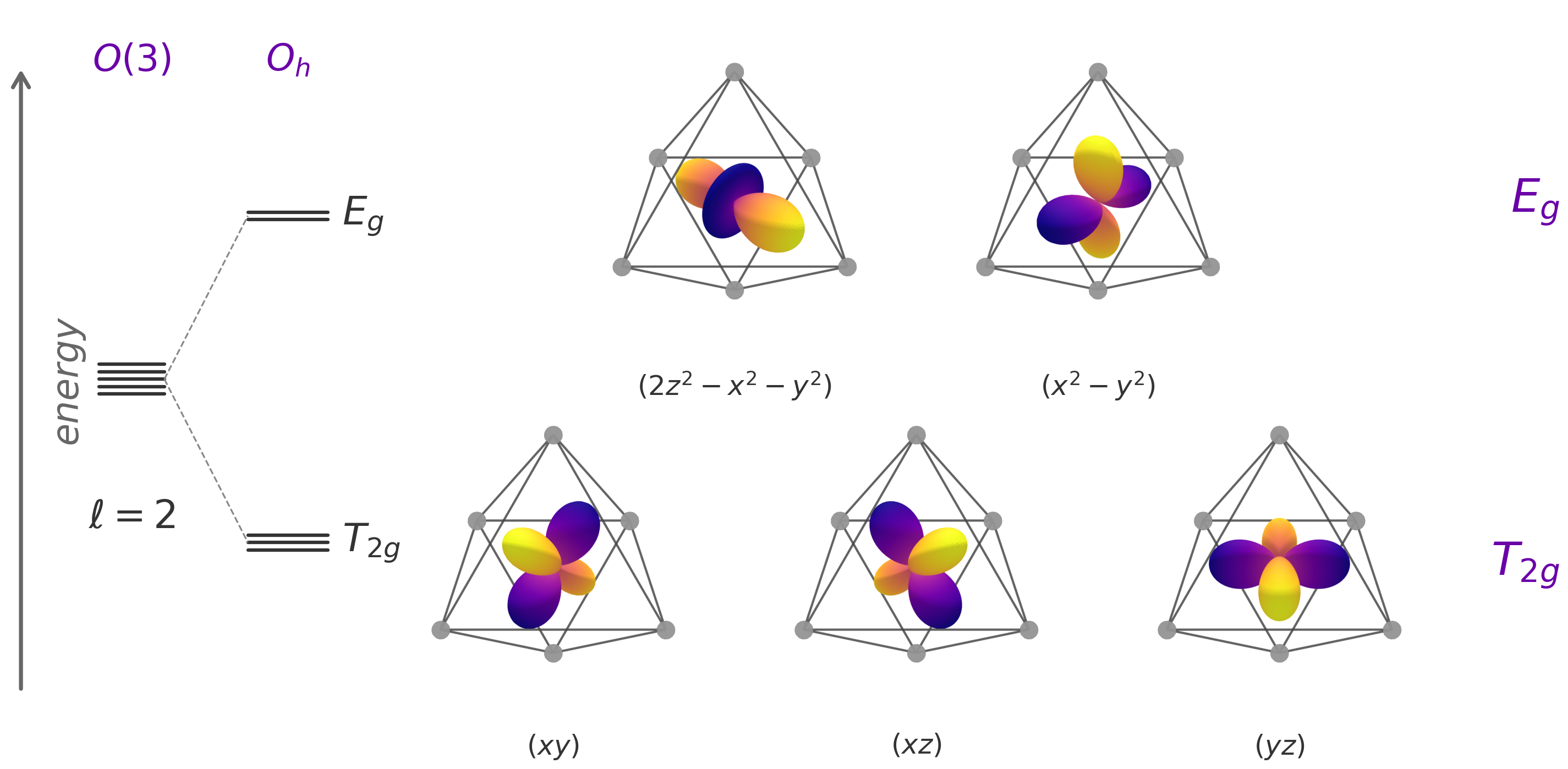
Who sits higher — E_g or T_{2g}? (A non-symmetry argument.) Symmetry alone tells you that l=2 branches as E_g \oplus T_{2g}: it gives you the partition into two degenerate levels, but not which one is higher in energy. Group theory is blind to this because both irreps are equally good invariant subspaces under O_h.
The ordering is a Coulombic result. The E_g orbitals (d_{z^2} and d_{x^2 - y^2}) have lobes pointing directly at the six octahedrally-coordinated ligands, so an electron in an E_g orbital feels strong electrostatic repulsion from the ligand electron density. The T_{2g} orbitals (d_{xy}, d_{xz}, d_{yz}) have lobes pointing between the ligands, so they feel much less. Higher repulsion ⇒ higher energy, so E_g sits above T_{2g} in an octahedral field. The split is the famous "10 Dq" or \Delta_o of ligand field theory, with E_g at +\tfrac{3}{5}\Delta_o and T_{2g} at -\tfrac{2}{5}\Delta_o relative to the energy of the (unsplit) \ell = 2 level.
In a tetrahedral field (T_d, ligands at 4 of the 8 body-diagonals of a cube) the geometry flips: it is now the t_2 orbitals (the tetrahedral analogues of T_{2g}) whose lobes point closer to the ligands, so e is lower and t_2 is higher. Same symmetry split, opposite ordering — a reminder that the geometry of the ligand field, not just the abstract group, is what sets the sign of the splitting.
The punchline. Every character table's basis function columns are determined by a single computation: branch the O(3) spherical harmonics to the point group's irreps. The branching table (previous subsection) contains all the information — the character table just presents it in a more familiar form with the polynomials written out explicitly. Higher-order columns (cubic, quartic, ...) follow from branching higher-l irreps.
6) Cartesian Tensors
6.1) Definition
A Cartesian tensor is a tensor whose indices span the orthogonal directions of Euclidean space (\hat{x}, \hat{y}, \hat{z}):
- Vector: V_i, i \in \{x, y, z\} — 3 components, 1 index
- Matrix: M_{ij}, i, j \in \{x, y, z\} — 9 components, 2 indices
- Order-n tensor: T_{i_1 i_2 \ldots i_n} — 3^n components, n indices
The number of tensor indices equals the order of the tensor (analogous to the order/degree of a polynomial).
6.2) Representation on Cartesian Tensors
Under a rotation/reflection g \in O(3), a Cartesian tensor transforms by "rotating each index" with the vector representation:
In code: np.einsum('ijk,ai,bj,ck->abc', T, rot_mat, rot_mat, rot_mat)
Equivalently, flatten the tensor to a 3^n-dimensional vector and apply the n-fold tensor product of the vector representation:
6.3) Index Symmetries Reduce Degrees of Freedom
Physical tensors often have symmetries on their indices — constraints like T_{ij} = T_{ji} or T_{ijk} = -T_{jik} — that reduce the number of independent components. These constraints come from the physics of the quantity being described (e.g. stress is symmetric because of torque balance), not from any rotation or point group symmetry. They act purely on the indices: permuting which entries are tied together, and possibly flipping signs.
The d.o.f. reduction from index symmetries happens before O(3) enters the picture. Only after we know which subspace the tensor lives in do we ask "how does this subspace decompose into O(3) irreps?" (next section) and "which of those irreps survive under a point group?" (branching).
General matrix M_{ij}: 9 d.o.f. (no index constraint).
Symmetric matrix M_{ij} = M_{ji}: 6 d.o.f. The constraint ties T_{xy} = T_{yx}, T_{xz} = T_{zx}, T_{yz} = T_{zy} (3 pairs), reducing 9 entries to 6 independent ones.
The elasticity tensor C^{ijkl} (order 4): a general order-4 tensor has 3^4 = 81 d.o.f. But the elasticity tensor T^{ij} = C^{ijkl} E_{kl} (relating stress to strain) has three symmetry constraints:
- ij = ji (stress tensor is symmetric)
- kl = lk (strain tensor is symmetric)
- ijkl = klij (from the elastic energy being a symmetric second derivative: C^{ijkl} = \frac{\partial^2 U}{\partial E_{ij} \partial E_{kl}})
These reduce the d.o.f. from 81 to 21.
The Levi-Civita tensor \epsilon_{ijk} (order 3, fully antisymmetric): ijk = -jik = -ikj. A general order-3 tensor has 3^3 = 27 d.o.f.; the full antisymmetry constraint leaves just 1 d.o.f. — a single independent entry (up to normalization).
The interactive graphic below visualizes these constraints. In the Grid tab, tensor entries that are tied together by the index symmetry share the same color — they are not independent, but constrained to be equal (or negated, depending on the sign). Entries forced to zero (because the symmetry maps them to their own negative) appear in gray. In the Basis tab, each basis vector shows the specific linear combination of entries that forms one independent degree of freedom — the signs (positive in orange, negative in purple) encode the \pm 1 sign requirements imposed by the permutation-and-sign formula.
7) Decomposing Cartesian Tensors into Irreps
7.1) Recipe: From Index Symmetry to Irrep Decomposition
Given a Cartesian tensor with index symmetries (e.g., "ij = ji" or "ijk = -jik"), how do we determine which irreps appear and how many degrees of freedom survive?
The key idea: an index symmetry like "ij = ji" imposes a constraint on the tensor entries. This constraint has two parts that act independently:
- Permutation: which entries get swapped (e.g., T_{xy} and T_{yx} swap positions)
- Sign: whether the swapped entries are equal (ij = ji) or negated (ij = -ji)
These are independent operations — the permutation acts on the locations of entries, while the sign acts on their values. Together they define which subspace of the full 3^n-dimensional tensor space the constrained tensor lives in.
7.2) Worked Example: The Levi-Civita Tensor (ijk = -jik)
The fully antisymmetric rank-3 tensor satisfies T_{ijk} = -T_{jik} = -T_{ikj}. Let's trace through what this means concretely.
Consider swapping the first two indices: ijk \to jik. This is a permutation (swap positions 1 and 2) combined with a sign flip (the - in ijk = -jik). On the 3^3 = 27 entries of the tensor:
- The permutation maps T_{xyz} \leftrightarrow T_{yxz}, T_{xzy} \leftrightarrow T_{zxy}, etc.
- The sign constraint says T_{xyz} = -T_{yxz} at each swapped pair
- Entries where both indices are equal (like T_{xxz}) must satisfy T_{xxz} = -T_{xxz}, so T_{xxz} = 0
The formula ijk = -jik = -ikj generates the full group of permutations and signs (the alternating group with signs — 6 elements). The invariant subspace under all these constraints has dimension 1: there is only one independent entry (up to normalization), and the tensor is proportional to the Levi-Civita symbol \epsilon_{ijk}. This single degree of freedom transforms as 0o (a pseudoscalar).
7.3) The General Recipe
The approach is analogous to what we did for vibrational modes: we have the full 3^n-dimensional representation of O(3) on the Cartesian tensor, but the index symmetry formula restricts us to some subspace. We project the O(3) representation onto that subspace, then decompose into irreps.
Step 1: Parse the symmetry formula into a permutation group and a sign group.
perm_rep, sign_rep = grids.formula_to_perm_and_sign_group('ij=ji')

# perm_rep.shape = (2, 2, 2) — two 2×2 permutation matrices (identity + swap)
# perm_rep[0] = [[1, 0], [0, 1]]  (identity: i,j → i,j)
# perm_rep[1] = [[0, 1], [1, 0]]  (swap:     i,j → j,i)
#
# sign_rep = [+1, +1] — both permutations have sign +1 (ij = +ji)
# For 'ij=-ji', sign_rep would be [+1, -1]
The perm_rep is a set of permutation matrices acting on the index positions (e.g., for a rank-2 tensor, swapping i \leftrightarrow j is a 2 \times 2 permutation matrix). The sign_rep is a matching set of \pm 1 values that tell you whether the permuted tensor is equal to (+1) or the negative of (-1) the original.
Why separate the permutation and sign? The permutation and sign together define the full action on the tensor: the permutation shuffles entry positions, and the sign flips values. Ultimately we need their tensor product (sign \times grid permutation) to find the invariant subspace. But when generating the group from the formula, it's much more convenient to work with the direct sum (block-diagonal) of the two representations. This way we can generate the full group from the formula's generators, then extract the permutation and sign components independently. The function formula_to_perm_and_sign_group does exactly this: it builds the group in the direct sum, then returns perm_rep and sign_rep separately so we can use them in the subsequent steps.
Step 2: Lift the index permutations to a permutation representation on the tensor entries.
grid_rep = grids.perm_to_grid_rep(perm_rep, [3, 3])
# grid_rep.shape = (2, 9, 9) — two 9×9 permutation matrices
The index permutation (a small n \times n matrix acting on index positions) gets lifted to a 3^n \times 3^n permutation matrix acting on the flattened tensor entries. You can think of the tensor as a 3^n-dimensional vector, and each index permutation becomes a 3^n \times 3^n permutation that shuffles entries. For example, swapping i \leftrightarrow j maps T_{xy} \leftrightarrow T_{yx}, T_{xz} \leftrightarrow T_{zx}, etc.
Step 3: Find the invariant subspace — the entries that satisfy the symmetry constraint.
new_basis, new_proj = grids.perm_and_sign_to_tensor_basis_and_proj(
    perm_rep, sign_rep, [3, 3]
)
# new_basis.shape = (6, 9) — 6 orthonormal basis vectors in 9-dim space
This function takes the grid permutation representation (from Step 2) and the sign representation (from Step 1), forms the projector P = \frac{1}{|G|}\sum_g s_g \cdot \pi_g (where s_g is the sign and \pi_g is the 3^n \times 3^n permutation matrix), then applies Gram-Schmidt to extract an orthonormal basis for the invariant subspace. For ij=ji (symmetric), this is a 6-dimensional subspace of the 9-dimensional space. For ij=-ji (antisymmetric), it's 3-dimensional.
Step 4: Project the O(3) tensor representation onto this subspace and decompose into irreps.
sub = np.einsum('ij,njk,kl->nil', new_basis, o3_tensor_rep, new_basis.T)
cob = [linalg.infer_change_of_basis(ir, sub) for ir in o3_irreps]
7.4) Examples
| Tensor | Symmetry | d.o.f. | Decomposition |
|---|---|---|---|
| General matrix M_{ij} | none | 9 | 0e \oplus 1e \oplus 2e |
| Symmetric matrix M_{ij} = M_{ji} | ij=ji |
6 | 0e \oplus 2e |
| Antisymmetric matrix M_{ij} = -M_{ji} | ij=-ji |
3 | 1e (pseudovector) |
Fully symmetric order-3 ijk=jik=ikj |
S₃ | 10 | 1o \oplus 3o |
Fully antisymmetric order-3 ijk=-jik=-ikj |
Alt₃ | 1 | 0o (pseudoscalar) |
7.5) Point Group Constraints on Tensor Components
The decomposition of a Cartesian tensor into O(3) irreps tells us which types of angular dependence the tensor can carry. But if the system has a point group symmetry (e.g. a crystal with symmetry group G \leq O(3)), then the branching rules from the previous section impose further constraints: only the components that transform as the trivial irrep (A_1) of G can be nonzero.
This is because a physical tensor property of the system (like the elasticity tensor of a crystal) must be invariant under the symmetry operations of the crystal. In representation-theoretic terms: the tensor must live in the A_1 subspace when branched to the point group.
Example: symmetric rank-2 tensor under T_d. The decomposition 0e \oplus 2e branches to T_d as:
- 0e \to A_1 (1 component — survives)
- 2e \to E \oplus T_2 (5 components — E and T_2 are NOT A_1, so they vanish)
So for a system with T_d symmetry, a symmetric rank-2 tensor has only 1 independent component (the isotropic/scalar part) out of the 6 allowed by index symmetry alone. The 5 traceless components are forced to zero by the point group.
General recipe: To determine the independent components of a Cartesian tensor for a system with point group G:
- Decompose the tensor into O(3) irreps (using index symmetry constraints)
- Branch each O(3) irrep to irreps of G (using the branching table)
- Count how many copies of A_1 (the trivial irrep of G) appear — this is the number of independent tensor components
This is the representation-theoretic explanation of why, for example, cubic crystals have only 3 independent elastic constants (out of 21 allowed by index symmetry), and why isotropic materials have only 2.
7.6) Connection to Spherical Harmonics
The polynomials generated by \bigotimes^n (x, y, z) with full symmetry (ijk\ldots = jik\ldots = \ldots) always contain exactly one copy of the highest-order irrep (l = n). This highest-order component is proportional to the degree-n spherical harmonics.
This gives an alternative route to constructing spherical harmonics: simply tensor product the l = 1 representation with itself n times, impose full index symmetry, and extract the highest-l irrep. Or even simpler — without the symmetry constraint, just take the outer product and extract the highest new irrep (the CG coefficients do the work for you).
7.7) Tensors in Physics and Engineering
Cartesian tensors appear everywhere:
- Gradient \nabla: a vector operator (
1o) - Laplacian \nabla^2 = \nabla \cdot \nabla: a scalar operator (
0e). Spherical harmonics are the solutions of \nabla^2 f = 0 that are spherically symmetric (homogeneous polynomials on the sphere). - Lorentz force \vec{F} = q(\vec{E} + \vec{v} \times \vec{B}): type-checking reveals \vec{E} is a vector (
1o), \vec{B} is a pseudovector (1e), and \vec{v} \times \vec{B} is a vector (1o) — consistent with \vec{F} being a vector. - Angular momentum \vec{L} = \vec{r} \times \vec{p}: a pseudovector (
1e), represented as an antisymmetric matrix L_{ij} = r_i p_j - r_j p_i.
8) Spectra of Spherical Signals
The procedure we followed for Cartesian tensors — take a tensor product representation, impose index symmetries, project onto an invariant subspace, and decompose into irreps — is completely general. It applies to any tensor product of representations with index symmetries, not just tensor products of the vector representation. Here we apply it to tensor products of spherical harmonic coefficients.
A signal on the sphere can be expanded in spherical harmonics: f(\hat{\mathbf{r}}) = \sum_{l,m} f_l^m \, Y_l^m(\hat{\mathbf{r}}). The coefficients f_l^m form a vector of dimension 2l + 1 for each l, transforming as the l-th irrep of \mathrm{SO}(3) under rotation. How do we build rotation-invariant descriptors from these coefficients?
8.1) Power Spectrum
The power spectrum is the simplest invariant: for each angular frequency l,
This is invariant because \sum_m |f_l^m|^2 is the squared norm of the l-th irrep component, and norms are preserved under unitary (orthogonal) transformations.
In the language of tensor products and index symmetries: the power spectrum is a symmetric rank-2 invariant of the SH coefficients. We form the tensor product f_l \otimes f_{l'}, impose the symmetry ll' = l'l (i.e. ij = ji), and project onto the scalar (l = 0) component. The CG coefficient for l \otimes l \to 0 is proportional to \delta_{mm'}, so the contraction gives \sum_m f_l^m f_l^m = P_l. This is exactly the same ij = ji index symmetry we saw for symmetric Cartesian tensors — but now applied to SH coefficients rather than spatial coordinates.
8.2) Bispectrum
The bispectrum is a rank-3 invariant: contract three sets of SH coefficients via CG coefficients to produce a scalar or pseudoscalar:
This is nonzero only when the triangle inequality |l_1 - l_2| \leq l_3 \leq l_1 + l_2 is satisfied (the CG selection rule). The output parity is (-1)^{l_1 + l_2 + l_3}: when the sum of angular momenta is even the result is a scalar (0e), when odd it is a pseudoscalar (0o). Both are rotation-invariant — the difference is their behavior under inversion. The bispectrum carries the fully symmetric rank-3 index symmetry l_1 l_2 l_3 = l_2 l_1 l_3 = l_1 l_3 l_2 — the same ijk = jik = ikj pattern as the fully symmetric Cartesian tensor from §6.
Connection to index symmetries. The power spectrum and bispectrum are not new mathematical objects — they are the same symmetric tensor contractions from §6, but applied to spherical harmonic coefficients instead of Cartesian coordinates. The power spectrum uses ij = ji (symmetric rank-2 \to scalar), the bispectrum uses ijk = jik = ikj (symmetric rank-3 \to scalar). Higher-order spectra (trispectrum, etc.) follow the same pattern with higher-rank fully symmetric index constraints.
The power spectrum captures the energy distribution across angular frequencies but loses phase information. The bispectrum captures phase correlations between triples of frequencies and is sufficient to reconstruct the signal up to rotation (for generic signals). Together, power spectrum + bispectrum form the basis of many rotation-invariant descriptors in molecular science, including SOAP (Bartók et al. 2013) and ACE (Drautz 2019).
9) Symmetrizing Spherical Harmonic Signals
9.1) Projecting onto the Invariant Subspace
Given a function on the sphere f(\hat{\mathbf{r}}) and a point group G \leq O(3), we can symmetrize f by averaging over the group:
The result \bar{f} is invariant under G by construction. In the spherical harmonic basis, this projection acts independently on each l-component: it projects the (2l+1)-dimensional coefficient vector f_l onto the subspace that transforms as the trivial irrep (A_1) of G within the l-th O(3) irrep.
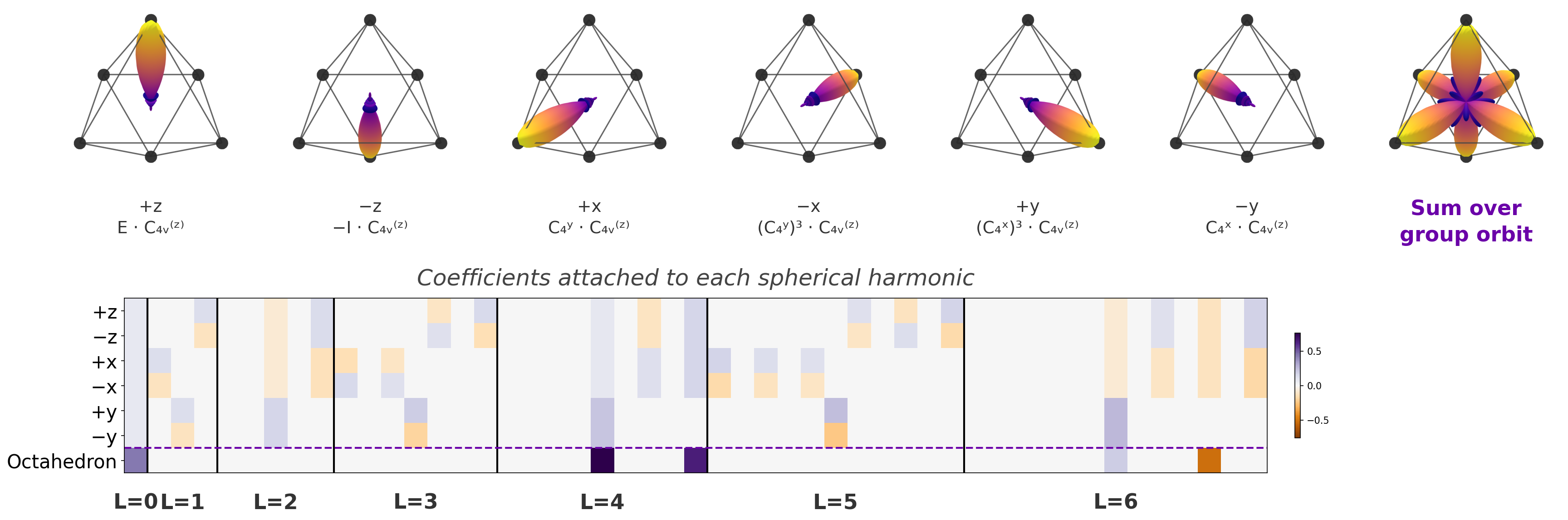
The graphic below demonstrates this for the octahedral group O_h. We place a single delta function at +\hat{z}, then hit it with every element of O_h and sum the results — the group orbit of +\hat{z} has only 6 distinct directions (the vertices of an octahedron, \pm x, \pm y, \pm z), because the stabilizer of +\hat{z} is the subgroup
of order |O_h|/6 = 8. Each of the other 5 vertices is reached by a single coset representative g_v, so the set of operations taking +\hat{z} to v is the coset g_v \cdot C_{4v}^{(z)}. The top row shows the SH expansion of each of the 6 deltas in the orbit (labeled by the coset that generates it) along with their sum; the bottom shows the SH coefficients grouped by l, where the octahedral sum retains only l = 0, 4, 6 — exactly the l-values whose branching under O_h contains the trivial irrep A_{1g}.
9.2) Which Spherical Harmonics Survive?
The branching table from §3 tells us exactly which l values have an A_1 component under G. If the branching of O(3) irrep le (or lo) under G does not contain A_1, then \bar{f}_l = 0 — the entire l-component is killed by symmetrization.
Example: O_h (octahedral/cubic symmetry). Looking at the branching table:
| O(3) irrep | Contains A_{1g}? | Survives? |
|---|---|---|
0e (l=0) |
Yes (A_{1g}) | ✓ (trivially — it's the constant) |
1o (l=1) |
No (T_{1u}) | ✗ |
2e (l=2) |
No (E_g + T_{2g}) | ✗ |
3o (l=3) |
No (A_{2u} + T_{1u} + T_{2u}) | ✗ |
4e (l=4) |
Yes (A_{1g} + E_g + T_{1g} + T_{2g}) | ✓ |
5o (l=5) |
No | ✗ |
6e (l=6) |
Yes (A_{1g} + A_{2g} + E_g + T_{1g} + 2T_{2g}) | ✓ |
The first non-trivial spherical harmonic that survives under O_h is l = 4. This means any function with octahedral symmetry, when expanded in spherical harmonics, has f_1 = f_2 = f_3 = 0 and the first nontrivial angular structure appears at l = 4 (a 9-dimensional space, of which only the 1D A_{1g} component is nonzero). This is why cubic harmonics start at l = 4 in crystal field theory.
9.3) Zeros in Spectra Under Symmetry
The symmetrization result directly predicts which spectral components vanish. If \bar{f}_l = 0 for some l (because branching has no A_1), then:
- The power spectrum P_l = \sum_m |\bar{f}_l^m|^2 = 0 for that l
- Any bispectrum entry B_{l_1 l_2 l_3} involving that l as any of l_1, l_2, l_3 is zero
The branching table is therefore a lookup table for spectral zeros: it predicts which entries of the power spectrum and bispectrum are forced to vanish for a signal with a given point group symmetry, without ever computing the signal itself.
10) Resources
- Dresselhaus, Group Theory: Application to the Physics of Condensed Matter, Ch. 6.3 — irreps of direct product groups
- Georgi, Lie Algebras in Particle Physics — \mathrm{SO}(3) and O(3) representations
- e3nn documentation —
Lpnotation and equivariant operations - Lie groups notes — generators, exponential parameterization, \mathrm{SO}(3) irreps
- Characters notes — character tables and their "linear/quadratic functions" columns
- Decomposition and products notes — tensor products, direct products, semi-direct products