Signals on Spheres and Spherical Convolution
Please Log In for full access to the web site.
Note that this link will take you to an external site (https://shimmer.mit.edu) to authenticate, and then you will be redirected back to this page.
These notes are being transcribed, condensed, and illustrated. They may lag or omit details, please refer to the handwritten notes for the full lecture.
1) Introduction and Roadmap
In the group convolution notes you saw convolution on finite groups — both the translation group \mathbb{Z}_N (where the irrep decomposition turned out to be the discrete Fourier transform) and non-abelian groups like D_4. The framework rested on three ideas:
- A vector space containing all functions on the group, with one coefficient per group element. (Formally, this is the regular representation.)
- Convolution in the irrep basis turned out to be diagonal. When we wrote group convolution in the irrep basis, we observed a striking structure: convolution couldn't mix different irreps, and within each irrep, the entire operation collapsed to a single scalar multiplication — one number per irrep, equal to the Fourier coefficient of the filter at that frequency. The convolution theorem — "convolution becomes pointwise multiplication in the Fourier basis" — is a restatement of this observed structure. (Formally, this is forced by Schur's lemma: any linear operation that commutes with the group action must be a scalar multiple of the identity within each irrep, so it can't do anything more interesting than a per-irrep rescaling.)
- A way to average over the group that respects the group action — for finite groups, "sum over all group elements and divide by |G|." This averaging is what makes the irrep matrix entries pairwise orthogonal, which in turn is what lets us extract Fourier coefficients by an inner product. (Formally, the Haar measure.)
This week we extend each of these ideas to a continuous group: \mathrm{SO}(3), the rotation group of 3D space. Each idea takes a new form:
- The "function on the group" vector space becomes infinite-dimensional — there are uncountably many rotations, so we can't store a coefficient at each one. The pivot in §3 is to a bandlimited irrep basis instead, parameterized by a finite number of coefficients per frequency.
- Equivariant operations still split the signal into independent irreps, but the irreps are now labeled by an integer l \geq 0 (each (2l+1)-dimensional) and the list is infinite. We choose a maximum l to make computations finite.
- The averaging operation becomes a continuous integral over the sphere S^2 or over \mathrm{SO}(3) itself, weighted by a measure that's invariant under group action.
The pivot we make in §3 is the key conceptual move: instead of representing functions on a continuous group element-by-element, we represent them in a bandlimited irrep basis. Two such bases will appear:
- Spherical harmonics Y_l^m(\hat{\mathbf{r}}) for signals on the sphere S^2 — introduced briefly in §2, drawing on the construction in the O(3) and spherical harmonics notes.
- Wigner D matrix entries D^l_{mn}(g) for signals on \mathrm{SO}(3) itself — introduced in §3.
With these two bases in hand, the central new operation of the week falls into place: spherical convolution (§6). Spherical convolution is the rotation-equivariant analog of ordinary 2D convolution — instead of sliding a filter over every possible translation of an image, we rotate a filter to every possible 3D orientation of a spherical signal, computing an inner product at each. Since rotations are parameterized by elements of \mathrm{SO}(3), the output naturally lives on \mathrm{SO}(3) and is expressed in the Wigner D basis from §3. This is the workhorse operation of spherical CNNs and the natural bridge between the group convolution framework on finite groups and the steerable convolution framework that uses irrep bases throughout.
Once the bases and the convolution operation are in place, the rest follows the script you already know from finite groups: bandwidth (§4), pointwise vs. tensor-product operations on signals (§5), and rotation-invariant descriptors built from tensor products with index symmetries (§7). The new content unique to the continuous case is the bispectrum inversion trick (§8), the relationship between point group symmetry and spectral zeros (§9), and the bandwidth-breaking activation trick (§20) that lets low-frequency irreps represent high-frequency signals.
2) Signals on the Sphere: Spherical Harmonics
A scalar signal on the sphere is a function
where \hat{\mathbf{r}} = (x, y, z) is a unit vector. Examples include a temperature map of the Earth, a charge density on a unit sphere around an atom, or a probability distribution over orientations.
Because spherical harmonics form a complete orthogonal basis for the space of square-integrable functions on S^2, any such signal can be expanded:
This is the continuous analog of the Wonderful Orthogonality Theorem: the irrep basis (here the spherical harmonics) decomposes any signal into rotation-covariant pieces. For the construction of Y_l^m as polynomials in (x, y, z) that transform as the l-th irrep of \mathrm{SO}(3), see the basis functions section of the O(3) and spherical harmonics notes.
2.1) Counting Coefficients
For each angular frequency l, there are 2l + 1 values of m (from -l to +l), giving a coefficient vector f_l \in \mathbb{R}^{2l+1}. Under rotation R \in \mathrm{SO}(3),
where D^l(R) is the (2l+1) \times (2l+1) Wigner D matrix — the irrep matrix of \mathrm{SO}(3) in the l-th representation. So f_l transforms as the l-th irrep, exactly as advertised.
If we bandlimit the signal at L_{\max} (drop all l > L_{\max}), the total number of real coefficients is
We'll need this count again in §3 when we compare to functions on \mathrm{SO}(3).
2.2) Real vs. Complex Basis
The course uses real spherical harmonics throughout (matching the Cartesian-monomial conventions in character tables and in e3nn). For the relationship to the complex basis Y_l^m \propto e^{im\phi} P_l^{|m|}(\cos\theta) from physics, see the real vs. complex basis discussion in the O(3) notes.
3) Signals on \mathrm{SO}(3): Wigner D Matrices
The story so far covers signals on S^2. But we may want to represent functions on the rotation group itself: f : \mathrm{SO}(3) \to \mathbb{R}. Examples include the result of cross-correlating a spherical filter with a spherical signal at every possible orientation (§6 below), or a probability distribution over 3D orientations of a molecule.
How do we represent such a function?
3.1) Why the Regular Rep Approach Doesn't Work
For finite groups, "function on the group" had a clean answer: reach for the regular representation. A function f : G \to \mathbb{R} on a finite group is just a vector in \mathbb{R}^{|G|} — one coefficient per group element. Group action becomes matrix multiplication by the regular representation matrix. This worked beautifully for \mathbb{Z}_N and for non-abelian finite groups like D_4.
For \mathrm{SO}(3), |G| = \infty. The regular representation is infinite-dimensional — there are uncountably many rotations, so we cannot store a coefficient at each. We need a different approach.
3.2) The Pivot: Irrep Basis with Finite Bandwidth
The solution is to work in the irrep basis with finite bandwidth — a Fourier expansion on the group. Instead of indexing by group elements (impossible for \mathrm{SO}(3)), we index by irreps:
The basis functions are the matrix entries D^l_{mn}(g) of the irreps, viewed as functions of g. By bandlimiting at L_{\max}, we get a finite parameterization of an arbitrary smooth function on \mathrm{SO}(3).
3.3) Aside: Groups as Manifolds, and Coset Spaces
Before going further, we need to be explicit about a Lie-group fact that's been hiding in plain sight: a Lie group is itself a manifold, and so are the spaces it acts on. The relationship between \mathrm{SO}(3) and the sphere S^2 is the relationship between two manifolds — not just between an abstract group and a "thing it acts on."
Recall from the Lie groups notes that a Lie group like \mathrm{SO}(2) or \mathrm{SO}(3) has a parameter manifold — a continuous parameterization by some number of real numbers (one angle for \mathrm{SO}(2), three Euler angles for \mathrm{SO}(3)). Up to topology, the parameter space is the group as a manifold:
- \mathrm{SO}(2) \cong S^1 as a manifold. Each rotation is specified by one angle \theta \in [0, 2\pi), with \theta = 0 and \theta = 2\pi identified. As a topological space, this is exactly a circle. So "signals on the circle" and "signals on \mathrm{SO}(2)" mean the same thing — one rotation per point on the circle.
- \mathrm{SO}(3) is a 3-dimensional manifold. Three Euler angles parameterize it (modulo the conventional periodicities and a global identification). This 3-manifold is not a sphere S^2 — the sphere is 2-dimensional. So signals on \mathrm{SO}(3) and signals on S^2 are genuinely different things, and we need a way to relate them.
Coset spaces. When a group G acts on a manifold M and the action is transitive (any point can be reached from any other by some group element), there's a clean way to identify M with a quotient of G. Pick a reference point p_0 \in M. The stabilizer
is the subgroup of elements that fix p_0. Two elements g, g' \in G send p_0 to the same point of M if and only if they differ by a stabilizer element (g^{-1} g' \in H). This identifies M with the coset space
— one coset per point of M.
For S^2 acted on by \mathrm{SO}(3): pick the north pole \hat{\mathbf{z}} as the reference. Its stabilizer is the subgroup of rotations that fix \hat{\mathbf{z}} — namely, the rotations about the z-axis, which form a copy of \mathrm{SO}(2) (call it \mathrm{SO}(2)_z).
To see why this leads to S^2 \cong \mathrm{SO}(3)/\mathrm{SO}(2)_z, work through the geometry concretely. Suppose we want to rotate \hat{\mathbf{z}} to some target direction \hat{\mathbf{p}} on the sphere. The rotation that does this is not unique. If g is any rotation with g \cdot \hat{\mathbf{z}} = \hat{\mathbf{p}}, then for every angle \theta \in [0, 2\pi), the composite rotation g \cdot R_z(\theta) also sends \hat{\mathbf{z}} to \hat{\mathbf{p}}:
because R_z(\theta) fixes \hat{\mathbf{z}} as the first step (it's an element of the stabilizer). In words: we can spin \hat{\mathbf{z}} about itself by any amount before applying the main rotation, and the destination on the sphere is completely unchanged. The "main rotation" g has no way to know whether such a pre-spin happened.
So the set of all rotations that send \hat{\mathbf{z}} to \hat{\mathbf{p}} is not a single rotation but an entire right coset — a one-parameter family parameterized by \theta:
To get a clean correspondence between "points on the sphere" and "rotations," we have to either pick one representative rotation from each coset (an arbitrary choice) or identify all rotations within a coset with their common destination. The latter is precisely the coset-space construction:
one point of the sphere per coset of \mathrm{SO}(2)_z inside \mathrm{SO}(3). The arbitrary "first spin about \hat{\mathbf{z}}" is exactly what gets quotiented out. The dimension count is consistent: \mathrm{SO}(3) is 3-dimensional, \mathrm{SO}(2) is 1-dimensional, the quotient is 3 - 1 = 2-dimensional, matching S^2.
A useful mental picture: \mathrm{SO}(3) sits over S^2 as a circle bundle — over each point of the sphere, there's a whole circle's worth of rotations (the coset), and the entire 3-manifold \mathrm{SO}(3) assembles from these one-dimensional fibers stacked over a two-dimensional base. The "extra" Wigner D modes with n \neq 0 in the next subsections will turn out to be functions that vary along these fibers, while the n = 0 modes are the ones that are constant along each fiber and therefore well-defined as functions on the sphere itself.
For S^1 acted on by \mathrm{SO}(2): the action is also transitive, but now the stabilizer of any point is just the trivial subgroup \{e\} (only the identity fixes a point), so
The "quotient by trivial subgroup" does nothing — the circle just is \mathrm{SO}(2) as a manifold.
The punchline that we'll use shortly: a function on G/H is the same as a function on G that's invariant under right-multiplication by H. (Two coset representatives of the same coset must give the same value, which is the right-H-invariance condition.) For S^2 = \mathrm{SO}(3)/\mathrm{SO}(2)_z, this means a spherical harmonic is a Wigner D function that's invariant under \hat{\mathbf{z}}-rotations — exactly the condition that picks out the n = 0 column of D^l in the deep-connection subsection below.
3.4) The \mathrm{SO}(2) Sanity Check
To see why the irrep-basis pivot is the natural extension of what we already know, look at \mathrm{SO}(2) (rotations of a circle). Functions on the circle expand in circular harmonics:
Here, e^{im\theta} plays both roles simultaneously: it's the basis function for signals on S^1 and the irrep matrix entry of \mathrm{SO}(2) at angle \theta. Two reasons they coincide:
- \mathrm{SO}(2) irreps are 1-dimensional, so the irrep "matrix" is just a scalar — no row or column index to distinguish.
- As we just saw, S^1 \cong \mathrm{SO}(2) as a manifold — the circle is the rotation group, no nontrivial coset to take. So "signal on the circle" and "signal on the group" are the same thing.
For \mathrm{SO}(3), neither simplification holds:
- Irreps are (2l+1)-dimensional, so D^l_{mn}(g) has two indices (m, n).
- S^2 \cong \mathrm{SO}(3) / \mathrm{SO}(2)_z is a proper coset space, so signals on S^2 are a strict subset of signals on \mathrm{SO}(3) — specifically, the right-\mathrm{SO}(2)_z-invariant ones.
These two structural differences are exactly what pulls spherical harmonics (signals on S^2) apart from Wigner D matrix entries (signals on \mathrm{SO}(3)).
3.5) Counting Basis Functions
The coefficient counts make this concrete:
| Group / domain | Basis functions | Coefficients per frequency |
|---|---|---|
| \mathrm{SO}(2), signals on S^1 | e^{im\theta} | 1 |
| \mathrm{SO}(2), signals on \mathrm{SO}(2) | e^{im\theta} | 1 |
| \mathrm{SO}(3), signals on S^2 | Y_l^m(\hat{\mathbf{r}}) | 2l + 1 |
| \mathrm{SO}(3), signals on \mathrm{SO}(3) | D^l_{mn}(g) | (2l+1)^2 |
The first two rows are identical because S^1 \cong \mathrm{SO}(2) — for \mathrm{SO}(2), the "sphere" and the group are the same space, so signals on the sphere and signals on the group are literally the same object. The split between the two only appears starting from \mathrm{SO}(3).
Bandlimited at L_{\max}, the totals scale as
- \mathrm{SO}(2), signals on S^1 or on \mathrm{SO}(2): 2L_{\max} + 1 (linear in L_{\max})
- \mathrm{SO}(3), signals on S^2: (L_{\max} + 1)^2 (quadratic)
- \mathrm{SO}(3), signals on \mathrm{SO}(3): \sum_l (2l+1)^2 = \tfrac{1}{3}(L_{\max}+1)(2L_{\max}+1)(2L_{\max}+3) (cubic)
The extra factor of 2l+1 in going from S^2 to \mathrm{SO}(3) is the price of working with a larger domain — \mathrm{SO}(3) has 3 angular dimensions vs. S^2's 2.
3.6) The Peter–Weyl Theorem
The statement that the matrix entries \{D^l_{mn}\} form a complete orthogonal basis for the space of square-integrable functions on \mathrm{SO}(3) is the Peter–Weyl theorem — the analog of the Wonderful Orthogonality Theorem for compact continuous groups. In the same way that WOT decomposed the regular representation of a finite group into irreps with multiplicity equal to dimension, Peter–Weyl says that the space of square-integrable functions on a compact group G decomposes as
where \widehat G is the set of irreps of G and d_\alpha is the dimension of irrep \alpha. For \mathrm{SO}(3), irrep l has dimension d_l = 2l + 1, so it appears in this decomposition with multiplicity 2l + 1 — giving exactly the (2l+1)^2 matrix entries D^l_{mn} we counted above. The finite-group story carries over verbatim, just with a sum over a (countably infinite but discrete) set of continuous-group irreps.
(A note on notation: the function-space L^2(X) is standard mathematical notation, but in physics we also use L^2 = L_x^2 + L_y^2 + L_z^2 for the squared angular momentum operator. To avoid clashing notation in these notes, we'll write out "square-integrable functions on X" rather than L^2(X).)
3.7) Parameterizing \mathrm{SO}(3): Euler Angles
To say anything concrete about D^l(g) we need a parameterization of g \in \mathrm{SO}(3). \mathrm{SO}(3) is a 3-dimensional Lie group, so any rotation can be written as a product of three elementary rotations about coordinate axes — Euler angles. The general form is
where a_1, a_2, a_3 \in \{x, y, z\} are axis labels. This compresses a 3 \times 3 orthogonal matrix (9 entries with 6 constraints) into 3 real numbers, which is the right count for a 3-dimensional manifold. Euler angles also play nicely with D^l: rotations about a single axis are easy to exponentiate (they act on the l-th irrep by \exp(\theta L_a^{(l)})), so the factorization above lets us evaluate D^l(g) as three matrix exponentials.
Many conventions exist. Different communities use different axis sequences:
- ZYZ (a_1 a_2 a_3 = z y z) is standard in quantum mechanics and most physics texts. The factorization is clean: D^l_{mn}(\alpha, \beta, \gamma) = e^{-im\alpha} d^l_{mn}(\beta) e^{-in\gamma}, with the two outer Z-rotations diagonal in the L_z eigenbasis and the small Wigner d-matrix d^l_{mn}(\beta) carrying all the nontrivial dependence.
- ZXZ is common in classical mechanics.
- ZYX ("yaw-pitch-roll") is standard in robotics and aerospace.
For practical reasons (compatibility with FFT-based spherical-harmonic evaluation; see the source e3nn/o3/_wigner.py and the wigner_D documentation), the e3nn library uses YXY:
with \gamma applied first, \beta second, \alpha third. In code, e3nn.o3.wigner_D(l, alpha, beta, gamma) returns the real D^l matrix in this convention.
The conceptual content is convention-independent — all valid Euler angle parameterizations cover \mathrm{SO}(3) and yield equivalent representations of D^l up to a change of basis. But the numerical values of coefficients depend on the convention, which becomes important the moment you write code.
Why we standardize on e3nn. Equivariance in code requires a consistent gauge — every operation in the network has to agree on what basis vectors of each irrep mean, what real-vs-complex SH convention is in use, what Euler angle ordering parameterizes a rotation, and so on. We don't currently know how to build modular code bases where each layer is allowed to "float" its gauge choice and still compose equivariantly. The pragmatic solution, used essentially everywhere in the equivariant-NN literature, is to standardize on a single library that fixes all these conventions at once. We use e3nn (real spherical harmonics, YXY Euler angles, specific irrep ordering) for this reason. Any code in this course that interacts with rotations or representations does so through e3nn's conventions; mixing libraries with different gauges silently breaks equivariance.
3.8) The Deep Connection: SH = Wigner D with One Euler Angle Fixed
There's a precise sense in which spherical harmonics are a slice of Wigner D. We illustrate it most cleanly in the ZYZ convention (the formulas below have analogs in YXY and other conventions; the geometry is the same).
In ZYZ Euler angles, the Wigner D matrix factors:
where d^l_{mn}(\beta) is the small Wigner d-matrix depending only on the second Euler angle. The two outer Z-rotations carry \alpha, \gamma dependence as pure phases (with frequencies m, n).
From the coset aside above: a function on the coset space S^2 \cong \mathrm{SO}(3) / \mathrm{SO}(2)_z is the same as a function on \mathrm{SO}(3) that is invariant under right-multiplication by elements of the stabilizer \mathrm{SO}(2)_z (i.e., rotations about \hat{\mathbf{z}}). Two rotations that differ by an \hat{\mathbf{z}}-rotation must be sent to the same value, because they correspond to the same point of the sphere.
In ZYZ Euler angles, this right-invariance condition has a particularly clean effect, because \gamma is itself the third Euler angle (the rightmost rotation in R_Z(\alpha) R_Y(\beta) R_Z(\gamma)). Composing on the right by an additional \hat{\mathbf{z}}-rotation R_Z(\gamma_0) just shifts the third Euler angle:
So invariance under right \hat{\mathbf{z}}-rotations is the same as saying f(\alpha, \beta, \gamma) doesn't depend on \gamma at all — it's a function of just (\alpha, \beta), the two angles that parameterize the sphere.
Now apply this condition to the Wigner D basis functions. The factorization above tells us the \gamma-dependence of D^l_{mn} is the pure phase factor e^{-in\gamma}, with frequency n. The only way e^{-in\gamma} is constant in \gamma for all \gamma is if n = 0. So the basis functions for S^2, viewed as a subset of basis functions for \mathrm{SO}(3), are exactly
— the n = 0 column of each Wigner D matrix, with the (now irrelevant) third angle pinned to \gamma = 0 as a coset representative.
Spherical harmonics are the n = 0 column of the Wigner D matrix. That's why they have 2l + 1 components instead of (2l+1)^2 — restricting from 3 angles to 2 collapses one matrix index. The remaining "extra" basis functions D^l_{mn} with n \neq 0 are the genuinely new degrees of freedom in the space of square-integrable functions on \mathrm{SO}(3) that don't exist on the sphere — they record how a signal varies along the fiber over each point of S^2 (i.e., how the signal changes as you spin the destination about itself).
In e3nn's YXY convention the same statement holds with the stabilizer subgroup pointing along \hat{\mathbf{y}} instead of \hat{\mathbf{z}} — the geometric coset S^2 \cong \mathrm{SO}(3) / \mathrm{SO}(2) is convention-independent, but which matrix index gets fixed depends on which axis the outer rotations point along.
4) Bandwidth on the Sphere
4.1) What "Bandwidth" Means Here
In the familiar 1D Fourier story, the bandwidth of a signal is the highest frequency |k| at which \hat f(k) has nonzero content. A signal is bandlimited at K if \hat f(k) = 0 for all |k| > K, in which case it lives in a finite-dimensional subspace of all functions on \mathbb{R}.
The spherical version is a direct analog: replace the continuous frequency |k| with the discrete angular frequency l \geq 0 that labels SH irreps. A signal f : S^2 \to \mathbb{R} is bandlimited at L_{\max} if f_l^m = 0 for all l > L_{\max}:
This is a finite-dimensional subspace of the square-integrable functions on S^2, of dimension (L_{\max} + 1)^2 — the count from §2. In code, "a spherical signal at bandwidth L_{\max}" is this array of (L_{\max}+1)^2 real coefficients.
Equivariant operations have predictable behavior on the bandwidth. Rotation, linear maps within an irrep, and group convolution all stay within the bandlimited subspace. Tensor products of two signals at bandwidths L_1 and L_2 may produce content up to L_1 + L_2 (CG selection rule). Pointwise nonlinearities (§20) are the exception: they generically create content at all higher l, which is precisely the mechanism we'll exploit to break the bandwidth limit.
4.2) Why Higher L_{\max} Gives Better Approximations
Two theorems are doing the work behind the intuition that "more l = better approximation":
Theorem (completeness of spherical harmonics). The spherical harmonics \{Y_l^m : l \geq 0,\ -l \leq m \leq l\} form a complete orthonormal basis of the square-integrable functions on S^2. For any square-integrable f, the SH expansion converges in mean square, and the truncation error is exactly the squared norm of the discarded coefficients:
where P_{L_{\max}} is the projection onto the bandlimited subspace. The proof is a special case of the Peter–Weyl theorem applied to the homogeneous space S^2 \cong \mathrm{SO}(3)/\mathrm{SO}(2). Further reading: Stein & Weiss, Introduction to Fourier Analysis on Euclidean Spaces, Ch. 4; or Atkinson & Han, Spherical Harmonics and Approximations on the Unit Sphere (2012), Ch. 2.
The completeness theorem says the SH expansion converges; the rate of convergence is governed by a second result.
Theorem (smoothness controls coefficient decay). The smoother the signal, the faster its SH coefficients decay, and therefore the smaller the truncation error at any given L_{\max}:
- Smooth functions (C^\infty): coefficients decay faster than any polynomial in l. The mean-square truncation error also decays faster than any polynomial in L_{\max} ("spectral accuracy").
- C^k functions (continuous derivatives up to order k): the mean-square truncation error scales as L_{\max}^{-k}.
- Analytic functions (locally given by convergent Taylor series): coefficients decay exponentially, |f_l^m| = O(e^{-cl}) for some c > 0. Truncation error decays exponentially in L_{\max}.
- Discontinuous or peaked functions (e.g. a delta function on the sphere): coefficients do not decay. For f(\hat{\mathbf{r}}) = \delta(\hat{\mathbf{r}} - \hat{\mathbf{r}}_0), |f_l^m|^2 = |Y_l^m(\hat{\mathbf{r}}_0)|^2, and \sum_m |Y_l^m(\hat{\mathbf{r}}_0)|^2 = (2l+1)/(4\pi) by the SH addition theorem — growing with l. Bandlimiting introduces O(1) error no matter how large L_{\max} is.
The takeaway: bandlimiting at L_{\max} is a good approximation precisely when the signal is smooth enough that the discarded high-l tail has small total mass. Further reading: Atkinson & Han Ch. 3 for precise rates and Sobolev-space formulations.
4.3) Angular Resolution and Spherical Nyquist
Combining these two theorems gives the operational rule. Spherical harmonics at frequency l have angular wavelength \sim 2\pi/l around a great circle, so to faithfully represent features of angular scale \theta (the size of a peak, the width of a coastline, the angular separation of two close peaks), you need
For example, an octahedrally-symmetric signal has peaks at \pm\hat{\mathbf{x}}, \pm\hat{\mathbf{y}}, \pm\hat{\mathbf{z}} separated by 90° = \pi/2, suggesting L_{\max} \gtrsim 2\pi/(\pi/2) = 4. This matches the result from the O(3) notes: l = 4 is the first nontrivial spherical harmonic frequency that survives the octahedral group O_h, so a non-constant octahedral signal cannot be represented at any L_{\max} < 4.
This is the spherical analog of the Nyquist–Shannon sampling theorem, and follows from a precise sampling result: a signal bandlimited at L_{\max} is uniquely determined by its values on a (2 L_{\max}) \times (2 L_{\max}) grid of latitudes and longitudes, with the grid spacing matched to the highest-frequency content the bandlimit allows. Beyond the bandlimit's resolution, signals become "indistinguishable" from smoother, lower-bandwidth versions under any rotation-equivariant probe. Further reading: Driscoll & Healy, Computing Fourier Transforms and Convolutions on the 2-Sphere, Advances in Applied Mathematics 15 (1994), 202–250.
For low-frequency signals (e.g. an octahedrally symmetric atomic environment, where the lowest nonzero l is 4 — see §9), bandlimiting at modest L_{\max} is essentially lossless. For high-frequency signals (Earth's coastlines, sharp probability distributions, near-delta functions), bandlimiting blurs the result and large L_{\max} is needed — or, alternatively, we can bring in nonlinearities to break the bandwidth limit (§20).
4.4) Bandwidth on \mathrm{SO}(3)
Everything above generalizes from S^2 to \mathrm{SO}(3) itself. A function f : \mathrm{SO}(3) \to \mathbb{R} expanded in Wigner D matrices is bandlimited at L_{\max} if \hat f^l_{mn} = 0 for l > L_{\max}. The total DOF is
— cubic in L_{\max}, vs. the quadratic count on S^2.
The three theorems carry over: Peter–Weyl gives completeness of \{D^l_{mn}\} in the space of square-integrable functions on \mathrm{SO}(3), smoothness controls the decay of \hat f^l_{mn}, and a \mathrm{SO}(3)-version of the sampling theorem gives a O(L_{\max}^3)-point grid that determines a bandlimited signal exactly. Further reading: Kostelec & Rockmore, FFTs on the Rotation Group (2008).
5) Operations on Signals: Pixel Products vs. Tensor Products
Once we represent signals as SH (or Wigner D) coefficients, we can ask: what are the natural operations? Two important ones, with a subtlety relating them.
5.1) Pointwise Multiplication on the Sphere
The most familiar operation is pointwise multiplication: given f, h : S^2 \to \mathbb{R}, form
This is symmetric: f \cdot h = h \cdot f. The product is again a function on the sphere, so it has its own SH expansion.
5.2) Tensor Product of Coefficients
In the irrep basis, multiplying signals corresponds to a tensor product of coefficient vectors. If f has coefficients f_l (transforming as irrep l) and h has coefficients h_{l'} (transforming as irrep l'), then f_l \otimes h_{l'} transforms as the tensor product representation, which decomposes via Clebsch–Gordan into
each summand a single irrep. Across all (l, l') pairs, the tensor product of two SH expansions gives a much larger object than the original signals.
5.3) Why Pointwise Product on S^2 Is "Smaller" Than Full Tensor Product
Here's the catch: pointwise multiplication on S^2 is commutative (f \cdot h = h \cdot f), so it can only realize the symmetric part of the tensor product. The antisymmetric paths (which would sense the order f \otimes h vs. h \otimes f) are killed by the symmetry of pointwise multiplication.
Concretely: the example x \cdot x = x^2 on the sphere. Both signals are identical (l = 1 vector), and the product is a degree-2 polynomial. The full tensor product 1 \otimes 1 contains 0 \oplus 1 \oplus 2 — the antisymmetric 1 (the cross product) is one of those paths, but it cannot appear in a pointwise product because the pointwise product is symmetric. The pixel product x \cdot x realizes only the symmetric paths 0 \oplus 2.
Paths matter. When we say "operate on signals" we always have to ask which paths through the tensor product we're realizing. Pointwise multiplication on S^2 realizes only the symmetric (commutative) paths. Convolution (§6) realizes a different subset. Power spectra and bispectra (§7) further restrict to scalar-output paths. Most equivariant neural network design comes down to choosing which paths to keep.
This phenomenon — that scalar-valued operations on S^2 realize only a subspace of the full tensor product algebra — is studied in detail in a recent series of papers (arXiv:2401.10216, arXiv:2506.13523, arXiv:2602.21466). For our purposes, the takeaway is that the irrep view is the complete picture; the pixel view is a projection of it.
6) Spherical Convolution
Convolution generalizes from finite groups to \mathrm{SO}(3) acting on signals on S^2. The setup: a signal f : S^2 \to \mathbb{R} and a filter \psi : S^2 \to \mathbb{R}, both on the sphere. The cross-correlation at orientation g is
The output is a function on \mathrm{SO}(3) — a scalar value at every possible orientation of the filter. This generalizes the regular-group convolution from the group convolution notes: there, the output was a function on the (finite) group; here, it's a function on \mathrm{SO}(3).
6.1) Real-Space Picture: A Permutation Representation on the Pixel Grid
Discretize the sphere as a grid of "pixels" \hat{\mathbf{r}}_1, \ldots, \hat{\mathbf{r}}_N. A signal becomes a vector in \mathbb{R}^N. The action of a rotation g \in \mathrm{SO}(3) permutes the pixels (approximately, for a generic grid): \psi(g^{-1} \hat{\mathbf{r}}_i) is just the value of \psi at a different grid point. So g acts on \mathbb{R}^N by a (signed) permutation matrix P(g). The "approximately" is necessary because rotations are continuous but the grid is discrete — for a generic rotation, the rotated pixel positions don't land exactly on grid points, and we have to interpolate.
A subtle point: this is not the regular representation of \mathrm{SO}(3). The regular representation of \mathrm{SO}(3) would be the action on functions on \mathrm{SO}(3) itself — the 3-dimensional manifold of all rotations. What we have here is the action of \mathrm{SO}(3) on functions on S^2, which is the smaller 2-dimensional coset space S^2 \cong \mathrm{SO}(3)/\mathrm{SO}(2)_z (§3). This is a permutation representation on the coset, not the regular rep. By the deep connection from §3, this representation contains each irrep L with multiplicity 1 (just the n = 0 column of D^L), not the multiplicity 2L+1 that the regular rep would give. This multiplicity-1 structure is exactly what produces the rank-1 outer-product form of the convolution theorem in the next subsection.
For \mathbb{Z}_N in the group convolution notes, the pixel set on the discretized circle was in bijection with \mathbb{Z}_N itself, so the permutation rep on pixels happened to coincide with the regular rep. For \mathrm{SO}(3) on S^2 that coincidence breaks — the pixel set is much smaller than the group.
In this real-space picture, cross-correlation is what it was for finite groups: a dot product of f with the rotated filter P(g)\psi, computed for every g. Schur's lemma (and hence the convolution-theorem block-diagonal structure) applies just as well to permutation reps on coset spaces as to the full regular rep — what changes is how much of each irrep block can be filled.
6.2) Fourier-Space Picture: Block-Diagonal in the Wigner D Basis
The output [f \star \psi](g) is a function on \mathrm{SO}(3), so by §3 it expands in the Wigner D basis:
The job of the convolution theorem is to compute these output Wigner D coefficients c_L^{mn} from the input SH coefficients \hat f_L^m and \hat \psi_L^n.
Derivation. Start from the integral. Expand the unrotated input f in spherical harmonics, and use the SH rotation rule for the rotated filter \psi:
The rotation rule says: under \hat{\mathbf{r}} \mapsto g^{-1} \hat{\mathbf{r}}, the SH coefficient vector \hat \psi_L transforms by the Wigner D matrix — the L-th irrep matrix — with no mixing across frequencies L.
Substitute into the integral and use orthonormality of SH, \int Y_{L'}^{m} Y_L^{n'} \, d\hat{\mathbf{r}} = \delta_{L L'} \delta_{m n'}:
Comparing to the Wigner D expansion at the top of this subsection, we read off the convolution theorem:
For each frequency L, the (2L+1) \times (2L+1) matrix c_L of output Wigner D coefficients is the outer product of the filter's SH coefficient vector and the signal's SH coefficient vector. The row index m comes from the filter; the column index n comes from the signal.
Two structural facts fall out:
- No cross-frequency mixing. c_L depends only on \hat f_L and \hat \psi_L — no coupling to coefficients at any other L' \neq L.
- Rank-one block within each frequency. c_L = \hat \psi_L \, \hat f_L^{\top} has rank one in the (m, n) indices — an outer product, not a generic (2L+1)^2 matrix. The cross-correlation can only produce this restricted family of Wigner D matrices.
This is Schur's lemma in action once again: cross-correlation is a linear, equivariant map from one \mathrm{SO}(3)-representation to another, so it must respect irrep decomposition. The block on irrep L is determined entirely by \hat f_L and \hat \psi_L — same structural story as the finite-group convolution theorem from L11–12, just with continuous irreps.
Convention notes for the formula. The boxed result c_L^{mn} = \hat \psi_L^m \hat f_L^n assumes (i) the cross-correlation convention [f \star \psi](g) = \int f(\hat{\mathbf{r}}) \psi(g^{-1} \hat{\mathbf{r}}) \, d\hat{\mathbf{r}}, (ii) the e3nn real Wigner D convention, and (iii) real spherical harmonics. With swapped naming or the opposite rotation in the integrand, the row/column indices swap; with complex spherical harmonics, a complex conjugate appears on one of the two SH coefficient vectors. The structural content — "block-diagonal in L, outer product in (m, n) within each block" — is convention-independent.
6.3) Reconciliation with the finite-group trace formulation
In the group convolution notes, the convolution theorem for non-abelian finite groups was written as a trace over the irrep matrix:
That trace is doing the same job as the double sum we just wrote. To see the equivalence, recall that the double sum over irrep matrix indices is a Frobenius product:
So our expansion [f \star \psi](g) = \sum_L \sum_{m, n} c_L^{mn} \, D^L_{mn}(g) is the same as \sum_L \text{tr}\big(C_L \, D^L(g)\big) with C_L = c_L^{\top}. Reading off "matrix coefficient C_L" versus expanding it elementwise as c_L^{mn} is just notation; the math is identical.
6.4) Why outer product instead of matrix product?
There's a sharper question lurking. For finite groups, the convolution theorem said \widehat{f \star \psi}^\alpha = \hat\psi_\alpha \hat f_\alpha^\dagger — a matrix product giving a generic d_\alpha \times d_\alpha matrix. Here, we ended up with an outer product C_L = \hat\psi_L \hat f_L^{\top} — a rank-1 matrix. Where did rank get lost?
The answer: inputs live on S^2, not on SO(3). By the deep connection in §3, a function on S^2, viewed as a function on SO(3), is supported entirely in the n = 0 column of D^L. So the "Fourier coefficient" of a spherical signal — viewed as an element of the Wigner D coefficient space on SO(3) — is not a generic matrix but a vector: the (2L+1) \times 1 column at n = 0.
Cross-correlating two such "vector inputs" produces an outer product \hat\psi_L \hat f_L^{\top}, which is a rank-1 matrix. This is a constraint on what the cross-correlation operation can produce, not a peculiarity of the formula: spherical convolution can only fill the rank-1 subspace of each Wigner D block.
If we instead had inputs that were already functions on \mathrm{SO}(3) (with full (2L+1) \times (2L+1) Fourier coefficient matrices), the convolution theorem would be a matrix product giving a full-rank output — just as in the finite-group case. The rank-1 / outer-product structure here is the signature of inputs living on a coset space rather than the full group.
| Convolution flavor | Input domain | Input Fourier coeffs | Output Fourier coeff per L | Theorem |
|---|---|---|---|---|
| Finite group G \times G \to G | functions on G | d_\alpha \times d_\alpha matrix | d_\alpha \times d_\alpha matrix | matrix product |
| SO(3): S^2 \times S^2 \to \mathrm{SO}(3) | functions on S^2 | (2L+1) \times 1 vector (n = 0 column) | (2L+1) \times (2L+1) matrix | outer product (rank 1) |
| SO(3): \mathrm{SO}(3) \times \mathrm{SO}(3) \to \mathrm{SO}(3) | functions on \mathrm{SO}(3) | (2L+1) \times (2L+1) matrix | (2L+1) \times (2L+1) matrix | matrix product |
Rows 1 and 3 are the same structural story: matrix product of full Fourier coefficients. Row 2 is the rank-1 specialization that arises specifically because the inputs live on a coset space. All three are forced by Schur's lemma: equivariant linear maps between SO(3)-representations must be block-diagonal in the irrep basis, and the dimension of each block (and how much of it is reachable via cross-correlation) depends on whether your inputs live on the group or on a coset.
6.5) Output as Scalars per Group Element
A common variant: instead of keeping the full output on \mathrm{SO}(3), project it back down to a function on S^2 by integrating over the third Euler angle \gamma. In the irrep view, this integration kills all the n \neq 0 Wigner D modes (which depend on \gamma as e^{-in\gamma} and integrate to zero over a full period) and keeps only the n = 0 column — which, by the deep connection in §3, is exactly the SH content. So this projected output is a spherical signal again, parameterized by (L_{\max}+1)^2 SH coefficients.
6.6) Equivariance
Spherical convolution is equivariant: rotating the input by h \in \mathrm{SO}(3) shifts the output by h,
This follows directly from the integration-by-substitution argument familiar from finite-group convolution (regular representation is equivariant by construction). The Fourier picture makes it manifest: the block-diagonal structure means rotation acts on each irrep block independently, and the output transforms as a function on \mathrm{SO}(3) in the Wigner D basis.
7) Power Spectra and Bispectra of Spherical Signals
The procedure we followed for Cartesian tensors — take a tensor product representation, impose index symmetries, project onto an invariant subspace, and decompose into irreps — is completely general. It applies to any tensor product of representations with index symmetries, not just tensor products of the vector representation. Here we apply it to tensor products of spherical harmonic coefficients.
A signal on the sphere can be expanded in spherical harmonics: f(\hat{\mathbf{r}}) = \sum_{l,m} f_l^m \, Y_l^m(\hat{\mathbf{r}}). The coefficients f_l^m form a vector of dimension 2l + 1 for each l, transforming as the l-th irrep of \mathrm{SO}(3) under rotation. How do we build rotation-invariant descriptors from these coefficients?
7.1) Power Spectrum
The power spectrum is the simplest invariant: for each angular frequency l,
This is invariant because \sum_m |f_l^m|^2 is the squared norm of the l-th irrep component, and norms are preserved under unitary (orthogonal) transformations.
In the language of tensor products and index symmetries: the power spectrum is a symmetric rank-2 invariant of the SH coefficients. We form the tensor product f_l \otimes f_{l'}, impose the symmetry ll' = l'l (i.e. ij = ji), and project onto the scalar (l = 0) component. The CG coefficient for l \otimes l \to 0 is proportional to \delta_{mm'}, so the contraction gives \sum_m f_l^m f_l^m = P_l. This is exactly the same ij = ji index symmetry we saw for symmetric Cartesian tensors — but now applied to SH coefficients rather than spatial coordinates.
7.2) Bispectrum
The bispectrum is a rank-3 invariant: contract three sets of SH coefficients via CG coefficients to produce a scalar or pseudoscalar:
This is nonzero only when the triangle inequality |l_1 - l_2| \leq l_3 \leq l_1 + l_2 is satisfied (the CG selection rule). The output parity is (-1)^{l_1 + l_2 + l_3}: when the sum of angular momenta is even the result is a scalar (0e), when odd it is a pseudoscalar (0o). Both are rotation-invariant — the difference is their behavior under inversion. The bispectrum carries the fully symmetric rank-3 index symmetry l_1 l_2 l_3 = l_2 l_1 l_3 = l_1 l_3 l_2 — the same ijk = jik = ikj pattern as the fully symmetric Cartesian tensor.
Connection to index symmetries. The power spectrum and bispectrum are not new mathematical objects — they are the same symmetric tensor contractions from the Cartesian tensors section of the O(3) notes, but applied to spherical harmonic coefficients instead of Cartesian coordinates. The power spectrum uses ij = ji (symmetric rank-2 \to scalar), the bispectrum uses ijk = jik = ikj (symmetric rank-3 \to scalar). Higher-order spectra (trispectrum, etc.) follow the same pattern with higher-rank fully symmetric index constraints.
The power spectrum captures the energy distribution across angular frequencies but loses phase information. The bispectrum captures phase correlations between triples of frequencies, and for many signals — depending on their specific structure — the power spectrum + bispectrum together are sufficient to reconstruct the signal up to rotation. This is not universally true, however: as we'll see in §8 below, there exist concrete counterexamples (adversarial point configurations) where the bispectrum fails to fully determine the signal. Despite this, power spectrum + bispectrum form the basis of many rotation-invariant descriptors in molecular science, including SOAP (Bartók et al. 2013) and ACE (Drautz 2019).
8) Bispectrum Inversion
The closing claim of §7 — that the bispectrum is sufficient to reconstruct the signal up to rotation — is striking, but how do we actually invert? Generic bispectrum inversion is hard. But for the kind of signals that appear in atomistic ML — sums of point masses on the sphere, representing neighbor positions — there's a clean algorithmic trick.
8.1) The Delta-Function Prior
Suppose we know f has the form
a weighted sum of delta functions on the sphere, representing N neighboring atoms at directions \hat{\mathbf{r}}_i with distances \|\vec r_i\|. Then the SH coefficients are
Given the bispectrum \{B_{l_1 l_2 l_3}\} and this prior (functional form known, atom count N unknown), we can often recover the atomic positions by an iterative procedure: alternately optimize candidate positions to match the bispectrum and merge nearby points (since two nearby atoms are indistinguishable from one atom of summed weight, in the angular signal).
Caveat: bispectrum is not always invertible. The "sufficient to reconstruct up to rotation" claim from §7 is a generic-signal statement, not a universal one. There exist specific configurations of points on the sphere — adversarial examples — that are not related by any rotation but produce identical bispectra. These configurations are indistinguishable to any descriptor based on three-body interactions (which is exactly what the bispectrum captures). See Pozdnyakov et al., Incompleteness of Atomic Structure Representations, Phys. Rev. Lett. 125, 166001 (2020) for explicit constructions of such adversarial point clouds. In practice, the bispectrum is invertible for "typical" environments encountered in real materials, but the existence of these counterexamples is important to keep in mind: bispectrum-based descriptors are not provably injective, only generically so.
8.2) Smoothness Under Distortion
Bispectrum descriptors degrade gracefully under distortion: small perturbations in atomic positions produce small changes in the bispectrum. This makes the bispectrum useful as a soft symmetry detector — the degree of (e.g.) octahedral symmetry of an environment becomes a continuous quantity rather than a binary yes/no.
8.3) Application: Clustering Local Atomic Environments
The bispectrum has been used to cluster local atomic environments in real materials databases. The general framework — including a bispectrum inversion algorithm and its use as an equivariant descriptor for atomic environments — is developed in Tuong Phung's MEng thesis (MIT, former TA for this course). As one demonstration from the broader line of work: the Ag environments in 669 crystals containing Ag–S bonds (3061 environments total) cluster into 8 distinct geometries — octahedron, tetrahedron, (bent) linear, T-shape, trigonal prism, seesaw, single neighbor, and trigonal planar — entirely from bispectrum features, without any human-supplied geometric labels.
For deeper coverage of bispectrum inversion and applications, see this Materials Project seminar talk.
9) Symmetrization and Spectral Zeros
"Lorsque certaines causes produisent certains effets, les éléments de symétrie des causes doivent se retrouver dans les effets produits." — Pierre Curie, Sur la symétrie dans les phénomènes physiques, symétrie d'un champ électrique et d'un champ magnétique (1894)
("When certain causes produce certain effects, the symmetry elements of the causes must be found in the effects produced.")
Curie's principle says that every symmetry element of a cause is preserved in its effect: if the cause is invariant under a group G, the effect must be too. In the language of representation theory, this becomes a precise lookup table: given the symmetry group G of a signal, the branching tables from the O(3) notes tell us which spherical harmonic coefficients must vanish — which in turn forces certain power spectrum and bispectrum entries to zero. For modern philosophical discussion, see Chalmers, Curie's Principle, BJPS 21, 133–148 (1970), and Castellani, On the meaning of symmetry breaking (in Brading & Castellani, eds., Symmetries in Physics: Philosophical Reflections, Cambridge University Press, 2003).
9.1) Projecting onto the Invariant Subspace
Given a function on the sphere f(\hat{\mathbf{r}}) and a point group G \leq O(3), we can symmetrize f by averaging over the group:
The result \bar{f} is invariant under G by construction. In the spherical harmonic basis, this projection acts independently on each l-component: it projects the (2l+1)-dimensional coefficient vector f_l onto the subspace that transforms as the trivial irrep (A_1) of G within the l-th O(3) irrep.
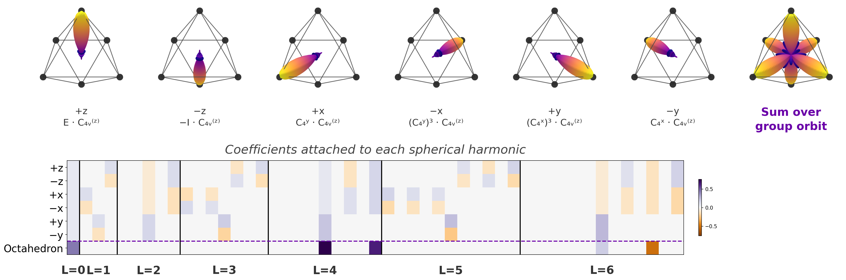
The graphic below demonstrates this for the octahedral group O_h. We place a single delta function at +\hat z, then hit it with every element of O_h and sum the results — the group orbit of +\hat z has only 6 distinct directions (the vertices of an octahedron, \pm x, \pm y, \pm z), because the stabilizer of +\hat z is the subgroup
of order |O_h|/6 = 8. Each of the other 5 vertices is reached by a single coset representative g_v, so the set of operations taking +\hat z to v is the coset g_v \cdot C_{4v}^{(z)}. The top row shows the SH expansion of each of the 6 deltas in the orbit (labeled by the coset that generates it) along with their sum; the bottom shows the SH coefficients grouped by l, where the octahedral sum retains only l = 0, 4, 6 — exactly the l-values whose branching under O_h contains the trivial irrep A_{1g}.
9.2) Which Spherical Harmonics Survive?
The branching table from the O(3) notes tells us exactly which l values have an A_1 component under G. If the branching of O(3) irrep le (or lo) under G does not contain A_1, then \bar{f}_l = 0 — the entire l-component is killed by symmetrization.
Example: O_h (octahedral/cubic symmetry). Looking at the branching table:
| O(3) irrep | Contains A_{1g}? | Survives? |
|---|---|---|
0e (l=0) |
Yes (A_{1g}) | ✓ (trivially — it's the constant) |
1o (l=1) |
No (T_{1u}) | ✗ |
2e (l=2) |
No (E_g + T_{2g}) | ✗ |
3o (l=3) |
No (A_{2u} + T_{1u} + T_{2u}) | ✗ |
4e (l=4) |
Yes (A_{1g} + E_g + T_{1g} + T_{2g}) | ✓ |
5o (l=5) |
No | ✗ |
6e (l=6) |
Yes (A_{1g} + A_{2g} + E_g + T_{1g} + 2T_{2g}) | ✓ |
The first non-trivial spherical harmonic that survives under O_h is l = 4. This means any function with octahedral symmetry, when expanded in spherical harmonics, has f_1 = f_2 = f_3 = 0 and the first nontrivial angular structure appears at l = 4 (a 9-dimensional space, of which only the 1D A_{1g} component is nonzero). This is why cubic harmonics start at l = 4 in crystal field theory.
9.3) Zeros in Spectra Under Symmetry
The symmetrization result directly predicts which spectral components vanish. If \bar{f}_l = 0 for some l (because branching has no A_1), then:
- The power spectrum P_l = \sum_m |\bar{f}_l^m|^2 = 0 for that l
- Any bispectrum entry B_{l_1 l_2 l_3} involving that l as any of l_1, l_2, l_3 is zero
The branching table is therefore a lookup table for spectral zeros: it predicts which entries of the power spectrum and bispectrum are forced to vanish for a signal with a given point group symmetry, without ever computing the signal itself. Curie's principle made operational.
10) Beating the Bandwidth Limit: Activations on the Sphere
Section 3 set up a tension: high-frequency signals (sharp Earth coastlines, peaked probability distributions) demand high L_{\max} to represent faithfully, which means more coefficients and more compute. Is there a way around it?
Yes — pointwise activation functions on the sphere, applied to a sum of multiple low-bandwidth SH signals, can produce arbitrarily high-frequency output.
10.1) The Setup
Replace a single bandlimited SH expansion with N independent bandlimited SH expansions, each with its own learnable coefficients f^{(i)}_l. Evaluate each on a grid on the sphere, apply a pointwise nonlinearity \sigma (e.g. SELU, softmax), and linearly combine:
The output g is a function on the sphere — but it is not bandlimited at L_{\max}. The pointwise nonlinearity introduces high-frequency content that wasn't in the input.
10.2) Why This Preserves Equivariance
Pointwise activation on the sphere is equivariant by construction: rotating the sphere then applying \sigma gives the same result as applying \sigma then rotating. So the operation respects the SO(3) action even though it produces frequencies above L_{\max}.
In the irrep view, equivariance is preserved because \sigma acts on the scalar field \sigma(f(\hat{\mathbf{r}})), which is a scalar function on the sphere — itself an SH-expandable signal, just with content at higher frequencies than the input had.
10.3) Why It Works (Universal Approximation)
A linear combination of N bandlimited SH signals with L_{\max} each spans a (N (L_{\max}+1)^2)-dimensional space of inputs to \sigma. Activations like SELU are nonlinear, and stacking enough of them gives universal approximation in the same sense as ordinary feed-forward networks — but here the "universal approximation" is over functions on the sphere, with equivariance baked in for free.
10.4) Example: Approximating Earth
A direct SH projection of a high-resolution Earth image at L_{\max} = 10 produces a blurry approximation. But N = 20 copies of L_{\max} = 10 SH each, passed through a SELU activation, then linearly combined, recovers a much sharper Earth — with the same total number of irrep coefficients. The nonlinearity is doing real work: it turns the low-frequency basis into a high-frequency representation.
This is the technique used in Symphony (Daigavane et al.) and related models for representing peaked angular distributions of next-atom positions in molecular generation.
11) Resources
Foundational papers
- Driscoll & Healy, Computing Fourier Transforms and Convolutions on the 2-Sphere, Advances in Applied Mathematics 15 (1994), 202–250
- Kostelec & Rockmore, FFTs on the Rotation Group (2008)
Spherical CNNs and equivariant networks
- Cohen et al., Spherical CNNs (ICLR 2018)
- Symphony — Appendix F (using multiple SH channels for high-frequency angular signals)
Bispectrum descriptors and atomic environments
- Bartók et al., SOAP (PRB 2013)
- Drautz, ACE (PRB 2019)
- Materials Project seminar: Applications of Bispectra in Materials ML
Pixel products vs. tensor products on the sphere
- Series of papers on scalar-valued operations on S^2 as a proper subspace of the full tensor product algebra: arXiv:2401.10216, arXiv:2506.13523, arXiv:2602.21466
Related notes
- Group Convolution — the finite-group version of everything in this note
- Steerable Convolution — the irrep-basis convolution framework that generalizes to continuous groups
- Lie Groups and Their Representations — the SO(3) irrep construction underlying Wigner D
- O(3) and Spherical Harmonics — SH construction, branching, Cartesian tensor index symmetries